33 Traditional IRT models
33.1 Terminology
Understanding IRT requires that we master some new terms. First, in IRT the underlying construct is referred to as theta or \(\theta\). Theta refers to the same construct we discussed in CTT, reliability, and our earlier measurement models. The underlying construct is the unobserved variable that we assume causes the behavior we observe in item responses. Different test takers are at different levels on the construct, and this results in them having different response patterns. In IRT we model these response patterns as a function of the construct theta. The theta scale is another name for the ability or trait scale.
Second, the dependent variable in IRT differs from CTT. The dependent variable is found on the left of the model, as in a regression or other statistical model. The dependent variable in the CTT model is the total observed score \(X\). The IRT model instead has an item score as the dependent variable. The model then predicts the probability of a correct response for a given item, denoted \(\Pr(X = 1)\).
Finally, in CTT we focus only on the person construct \(T\) within the model itself. The dependent variable \(X\) is modeled as a function of \(T\), and whatever is left over via \(E\). In IRT, we include the construct, now \(\theta\), along with parameters for the item that characterize its difficulty, discrimination, and lower-asymptote.
In the discussion that follows, we will frequently use the term function. A function is simply an equation that produces an output for each input we supply to it. The CTT model could be considered a function, as each \(T\) has a single corresponding \(X\) that is influenced, in part, by \(E\). The IRT model also produces an output, but this output is now at the item level, and it is a probability of correct response for a given item. We can plug in \(\theta\), and get a prediction for the performance we’d expect on the item for that level on the construct. In IRT, this prediction of item performance depends on the item as well as the construct.
The IRT model for a given item has a special name in IRT. It’s called the item response function (IRF), because it can be used to predict an item response. Each item has its own IRF. We can add up all the IRF in a test to obtain a test response function (TRF) that predicts not item scores but total scores on the test.
Two other functions, with corresponding equations, are also commonly used in IRT. One is the item information function (IIF). This gives us the predicted discriminatory power of an item across the theta scale. Remember that, as CTT discrimination can be visualized with a straight line, the discrimination in IRT can be visualized with a curve. This curve is flatter at some points than others, indicating the item is less discriminating at those points. In IRT, information tells us how the discriminating power of an item changes across the theta scale. IIF can also be added together to get an overall test information function (TIF).
The last IRT function we’ll discuss here gives us the SEM for our test. This is called the test error function (TEF). As with all the other IRT functions, there is an equation that is used to estimate the function output, in this case, the standard error of measurement, for each point on the theta scale.
This overview of IRT terminology should help clarify the benefits of IRT over CTT. Recall that the main limitations of CTT are: 1) sample and test dependence, where our estimates of construct levels depend on the items in our test, and our estimates of item parameters depend on the construct levels for our sample of test takers; and 2) reliability and SEM that do not change depending on the construct. IRT addresses both of these limitations. The IRT model estimates the dependent variable of the model while accounting for both the construct and the properties of the item. As a result, estimates of ability or trait levels and item analysis statistics will be sample and test independent. This will be discussed further below. The IRT model also produces, via the TEF, measurement error estimates that vary by theta. Thus, the accuracy of a test depends on where the items are located on the construct.
Here’s a recap of the key terms we’ll be using throughout this module:
- Theta, \(\theta\), is our label for the construct measured for people.
- \(\Pr(X = 1)\) is the probability of correct response, the outcome in the IRT model. Remember that \(X\) is now an item score, as opposed to a total score in CTT.
- The IRF is the visual representation of \(\Pr(X = 1)\), showing us our predictions about how well people will do on an item based on theta.
- The logistic curve is the name for the shape we use to model performance via the IRF. It is a curve with certain properties, such as horizontal lower and upper asymptotes.
- The properties of the logistic curve are based on three item parameters, \(a\), \(b\), and \(c\), which are the item discrimination, difficulty, and lower-asymptote, also known as the pseudo-guessing parameter.
- Functions are simply equations that produce a single output value for each value on the theta scale. IRT functions include the IRF, TRF, IIF, TIF, and TEF.
- Information refers to a summary of the discriminating power provided by an item or test.
33.2 The IRT models
We’ll now use the terminology above to compare three traditional IRT models. Equation (33.1) contains what is referred to as the three-parameter IRT model, because it includes all three available item parameters. The model is usually labeled 3PL, for 3 parameter logistic. As noted above, in IRT we model the probability of correct response on a given item (\(\Pr(X = 1)\)) as a function of person ability (\(\theta\)) and certain properties of the item itself, namely: \(a\), how well the item discriminates between low and high ability examinees; \(b\), how difficult the item is, or the construct level at which we’d expect people to have a probability \(\Pr = 0.50\) of getting the keyed item response; and \(c\), the lowest \(\Pr\) that we’d expect to see on the item by chance alone.
\[\begin{equation} \Pr(X = 1) = c + (1 - c)\frac{e^{a(\theta - b)}}{1 + e^{a(\theta - b)}} \tag{33.1} \end{equation}\]
The \(a\) and \(b\) parameters should be familiar. They are the IRT versions of the item analysis statistics from CTT, presented in Module 38.3. The \(a\) parameter corresponds to ITC, where larger \(a\) indicate larger, better discrimination. The \(b\) parameter corresponds to the opposite of the \(p\)-value, where a low \(b\) indicates an easy item, and a high \(b\) indicates a difficult item; higher \(b\) require higher \(\theta\) for a correct response. The \(c\) parameter should then be pretty intuitive if you think of its application to multiple-choice questions. When people low on the construct guess randomly on a multiple-choice item, the \(c\) parameter attempts to capture the chance of getting the item correct. In IRT, we acknowledge with the \(c\) parameter that the probability of correct response may never be zero. The smallest probability of correct response produced by Equation (33.1) will be \(c\).
To better understand the IRF in Equation (33.1), focus first on the difference we take between theta and item difficulty, in \((\theta - b)\). Suppose we’re using a cognitive test that measures some ability. If someone is high ability and taking a very easy item, with low \(b\), we’re going to get a large difference between theta and \(b\). This large difference filters through the rest of the equation to give us a higher prediction of how well the person will do on the item. This difference is multiplied by the discrimination parameter, so that, if the item is highly discriminating, the difference between ability and difficulty is magnified. If the discrimination is low, for example, 0.50, the difference between ability and difficulty is cut in half before we use it to determine probability of correct response. The fractional part and the exponential term represented by \(e\) serve to make the straight line of ITC into a nice curve with a lower and upper asymptote at \(c\) and 1. Everything on the right side of Equation (33.1) is used to estimate the left side, that is, how well a person with a given ability would do on a given item.
Figure 33.1 contains IRF for five items with different item parameters. Let’s examine the item with the IRF shown by the black line. This item would be considered the most difficult of this set, as it is located the furthest to the right. We only begin to predict that a person will get the item correct once we move past theta 0. The actual item difficulty, captured by the \(b\) parameter, is 3. This is found as the theta required to have a probability of 0.05 of getting the keyed response. This item also has the highest discrimination, as it is steeper than any other item. It is most useful for distinguishing between probabilities of correct response around theta 3, its \(b\) parameter; below and above this value, the item does not discriminate as well, as the IRF becomes more horizontal. Finally, this item appears to have a lower-asymptote of 0, suggesting test takers are likely not guessing on the item.
# Make up a, b, and c parameters for five items
# Get IRF using the rirf() function from epmr and plot
# rirf() will be demonstrated again later
ipar <- data.frame(a = c(2, 1, .5, 1, 1.5),
  b = c(3, 2, -.5, 0, -1),
  c = c(0, .2, .25, .1, .28),
  row.names = paste0("item", 1:5))
ggplot(rirf(ipar), aes(theta)) + scale_y_continuous("Pr(X)") +
  geom_line(aes(y = item1), col = 1) +
  geom_line(aes(y = item2), col = 2) +
  geom_line(aes(y = item3), col = 3) +
  geom_line(aes(y = item4), col = 4) +
  geom_line(aes(y = item5), col = 5)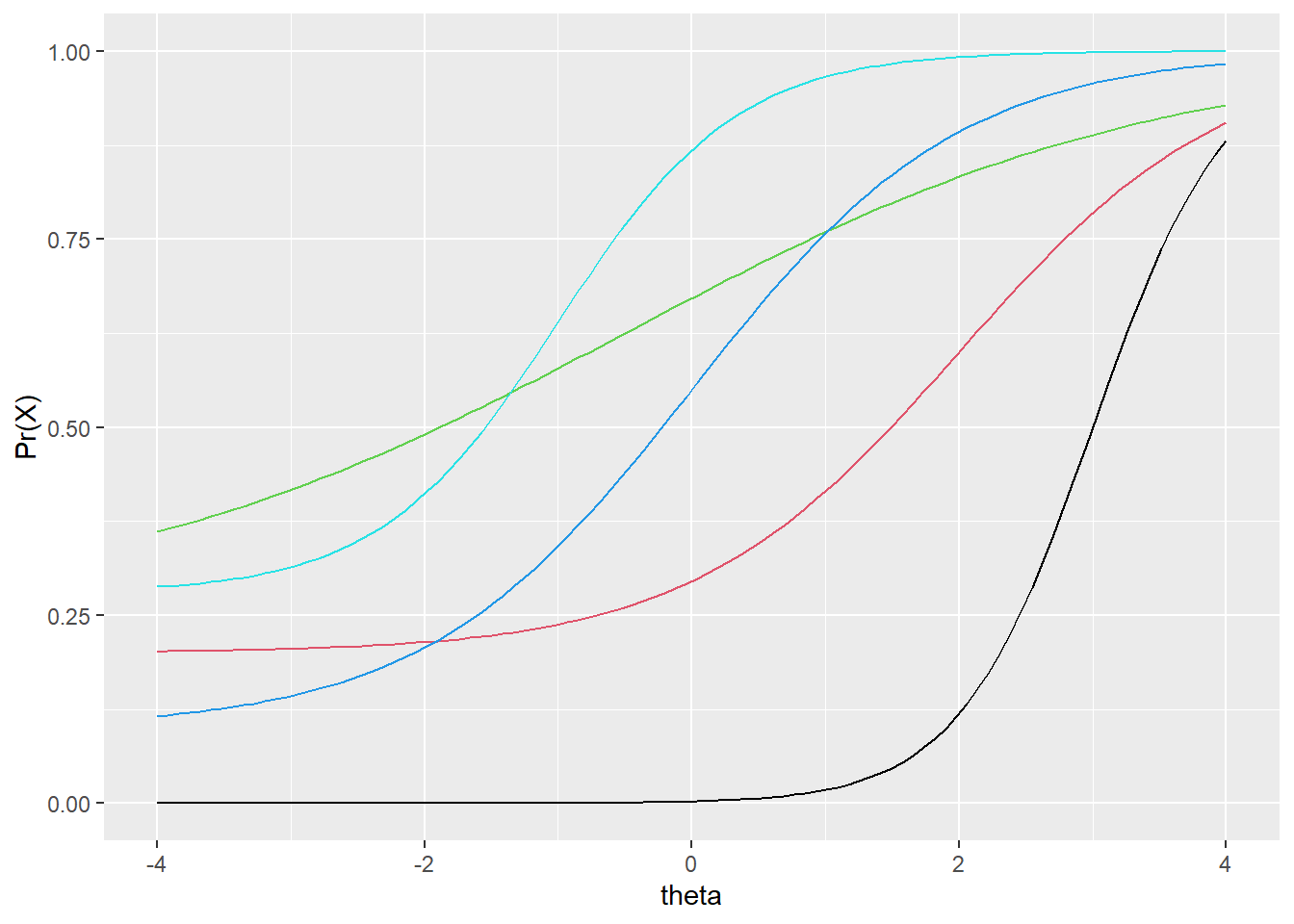
Figure 33.1: Comparison of five IRF having different item parameters.
Examine the remaining IRF in Figure 33.1. You should be able to compare the items in terms of easiness and difficulty, low and high discrimination, and low and high predicted probability of guessing correctly. Below are some specific questions and answers for comparing the items.
- Which item has the highest discrimination? Black, with the steepest slope.
- Which has the lowest discrimination? Green, with the shallowest slope.
- Which item is hardest, requiring the highest ability level, on average, to get it correct? Black, again, as it is furthest to the right.
- Which item is easiest? Cyan, followed by green, as they are furthest to the left.
- Which item are you most likely to guess correct? Green, cyan, and red appear to have the highest lower asymptotes.
Two other traditional, dichotomous IRT models are obtained as simplified versions of the three-parameter model in Equation (33.1). In the two-parameter IRT model or 2PL, we remove the \(c\) parameter and ignore the fact that guessing may impact our predictions regarding how well a person will do on an item. As a result,
\[\begin{equation} \Pr(X = 1) = \frac{e^{a(\theta - b)}}{1 + e^{a(\theta - b)}}. \tag{33.2} \end{equation}\]
In the 2PL, we assume that the impact of guessing is negligible. Applying the model to the items shown in Figure 33.1, we would see all the lower asymptotes pulled down to zero.
In the one-parameter model or 1PL, and the Rasch model (Rasch 1960), we remove the \(c\) and \(a\) parameters and ignore the impact of guessing and of items having differing discriminations. We assume that guessing is again negligible, and that discrimination is the same for all items. In the Rasch model, we also assume that discrimination is one, that is, \(a = 1\) for all items. As a result,
\[\begin{equation} \Pr(X = 1) = \frac{e^{(\theta - b)}}{1 + e^{(\theta - b)}}. \tag{33.3} \end{equation}\]
Zero guessing and constant discrimination may seem like unrealistic assumptions, but the Rasch model is commonly used operationally. The PISA studies, for example, utilize a form of Rasch modeling. The popularity of the model is due to its simplicity. It requires smaller sample sizes (100 to 200 people per item may suffice) than the 2PL and 3PL (requiring 500 or more people). The theta scale produced by the Rasch model can also have certain desirable properties, such as consistent score intervals (see de Ayala 2009).
33.3 Assumptions
The three traditional IRT models discussed above all involve two main assumptions, both of them having to do with the overall requirement that the model we chose is “correct” for a given situation. This correctness is defined based on 1) the dimensionality of the construct, that is, how many constructs are causing people to respond in a certain way to the items, and 2) the shape of the IRF, that is, which of the three item parameters are necessary for modeling item performance.
In Equations (33.1), (33.2), and (33.3) we have a single \(\theta\) parameter. Thus, in these IRT models we assume that a single person attribute or ability underlies the item responses. As mentioned above, this person parameter is similar to the true score parameter in CTT. The scale range and values for theta are arbitrary, so a \(z\)-score metric is typically used. The first IRT assumption then is that a single attribute underlies the item response process. The result is called a unidimensional IRT model.
The second assumption in IRT is that we’ve chosen the correct shape for our IRF. This implies that we have a choice regarding which item parameters to include, whether only \(b\) in the 1PL or Rasch model, \(b\) and \(a\) in the 2PL, or \(b\), \(a\), and \(c\) in the 3PL. So, in terms of shape, we assume that there is a nonlinear relationship between ability and probability of correct response, and this nonlinear relationship is captured completely by up to three item parameters.
Note that anytime we assume a given item parameter, for example, the \(c\) parameter, is unnecessary in a model, it is fixed to a certain value for all items. For example, in the Rasch and two-parameter IRT models, the \(c\) parameter is typically fixed to 0, which means we are assuming that guessing is not an issue. In the Rasch model we also assume that all items discriminate in the same way, and \(a\) is fixed to 1; then, the only item parameter we estimate is item difficulty.