22 Measurement models

In previous modules, we referred to unobserved variables as constructs. These somewhat metaphysical thingamajigs returned as the true score in classical test theory (Module 38.3). And we will see them again in the latent trait in item response theory (Module 31). The term factor is synonymous with construct, and refers to an underlying and unobservable trait, characteristic, or attribute assumed to cause or give rise to the observable behavior we measure and score using test items.

So, we now have three terms, construct, latent trait, and factor, that all refer essentially to the same thing, the underlying, unobserved variable of interest that we expect is causing people to differ in their test scores.

The constructs that we encounter in factor analysis, which we will refer to as factors, are qualitatively the same as the ones we encountered with CTT and IRT. In fact, the CTT and IRT models presented in this book could be considered special, focused applications of factor analysis within situations where we assume that a single construct is sufficient for explaining the correlations among observed variables, our test items. In CTT and IRT, we use a measurement model to summarize the similarities in scores across multiple items in terms of a single unobserved variable, the true score or theta, which we identify as the cause or source of variability in scores.

Factor analysis can be used more generally to identify multiple unobserved variables, or factors, that explain the correlations among our observed variables. So, the primary distinction between factor analysis and the measurement models we’ve seen so far is in the number of factors. The main objective of factor analysis within educational and psychological measurement is to explore the optimal reduced number of factors required to represent a larger number of observed variables, in this case, dichotomous or polytomous test scores.

Note the emphasis here on the number of factors being smaller than the number of observed variables. Factor analysis is a method for summarizing correlated data, for reducing a set of related observed variables to their essential parts, the unobserved parts they share in common. We cannot analyze more factors than we have observed variables. Instead, we’ll usually aim for the simplest factor structure possible, that is, the fewest factors needed to capture the gist of our data.

In testing applications, factor analysis will often precede the use of a more specific measurement model such as CTT or IRT. In addition to helping us summarize correlated data in terms of their underlying essential components, factor analysis also tells us how our items relate to or load on the factors we analyze. When piloting a test, we might find that some items relate more strongly to one factor than another. Other items may not relate well to any of the identified factors, and these might be investigated further and perhaps removed from the test. After the factor analysis is complete, CTT or IRT could then be used to evaluate the test further, and to estimate test takers’ scores on the construct. In this way, factor analysis serves as a tool for examining the different factors underlying our data, and refining our test to include items that best assess the factors we’re interested in measuring.

We’ll dig deeper into classical item analysis in Module 26, but what you need to know now it that it can also be used to refine a test based on features such as item difficulty and discrimination. Discrimination in CTT, which resembles the slope parameter in IRT, is similar to a factor loading in factor analysis. A factor loading is simply an estimate of the relationship between a given item and a given factor. Again, the main difference in factor analysis is that we’ll often examine multiple factors, and the loadings of items on each one, rather than a single factor as in CTT.

The model in Figure 22.1 contains a visual representation of a factor analysis where two factors are estimated to cause observed responses across a set of items. Remember that unidirectional arrows denote causal relationships. The underlying constructs, in ovals, are assumed to cause the observed item responses, in boxes. Bidirectional arrows denote correlations, where there is no clear cause and effect. The two factors, labeled Factor A and Factor B, each show a causal relationship with responses on all six items. Thus, each item is estimated to load on each factor. This is a unique feature of exploratory factor analysis, discussed next.

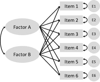
Figure 22.1: A simple exploratory factor analysis model for six items loading on two correlated factors.