13 Reliability study designs

Now that we’ve established the more common estimates of reliability and unreliability, we can discuss the four main study designs that allow us to collect data for our estimates. These designs are referred to as internal consistency, equivalence, stability, and equivalence/stability designs. Each design produces a corresponding type of reliability that is expected to be impacted by different sources of measurement error.

The four standard study designs vary in the number of test forms and the number of testing occasions involved in the study. Until now, we’ve been talking about using two test forms on two separate administrations. This study design is found in the lower right corner of Table 13.1, and it provides us with an estimate of equivalence (for two different forms of a test) and stability (across two different administrations of the test). This study design has the potential to capture the most sources of measurement error, and it can thus produce the lowest estimate of reliability, because of the two factors involved. The more time that passes between administrations, and as two test forms differ more in their content and other features, the more error we would expect to be introduced. On the other hand, as our two test forms are administered closer in time, we move from the lower right corner to the upper right corner of Table 13.1, and our estimate of reliability captures less of the measurement error introduced by the passage of time. We’re left with an estimate of the equivalence between the two forms.

As our test forms become more and more equivalent, we eventually end up with the same test form, and we move to the first column in Table 13.1, where one of two types of reliability is estimated. First, if we administer the same test twice with time passing between administrations, we have an estimate of the stability of our measurement over time. Given that the same test is given twice, any measurement error will be due to the passage of time, rather than differences between the test forms. Second, if we administer one test only once, we no longer have an estimate of stability, and we also no longer have an estimate of reliability that is based on correlation. Instead, we have an estimate of what is referred to as the internal consistency of the measurement. This is based on the relationships among the test items themselves, which we treat as miniature alternate forms of the test. The resulting reliability estimate is impacted by error that comes from the items themselves being unstable estimates of the construct of interest.

Table 13.1: Four Main Reliability Study Designs
	1 Form	2 Forms
1 Occasion	Internal Consistency	Equivalence
2 Occasions	Stability	Equivalence & Stability

Internal consistency reliability is estimated using either coefficient alpha or split-half reliability. All the remaining cells in Table 13.1 involve estimates of reliability that are based on correlation coefficients.

Table 13.1 contains four commonly used reliability study designs. There are others, including designs based on more than two forms or more than two occasions, and designs involving scores from raters, discussed below.

13.1 Interrater reliability

It was like listening to three cats getting strangled in an alley.
— Simon Cowell, disparaging a singer on American Idol

Interrater reliability can be considered a specific instance of reliability where inconsistencies are not attributed to differences in test forms, test items, or administration occasions, but to the scoring process itself, where humans, or in some cases computers, contribute as raters. Measurement with raters often involves some form of performance assessment, for example, a stage performance within a singing competition. Judgment and scoring of such a performance by raters introduces additional error into the measurement process. Interrater reliability allows us to examine the negative impact of this error on our results.

Note that rater error is another factor or facet in the measurement process. Because it is another facet of measurement, raters can introduce error above and beyond error coming from sampling of items, differences in test forms, or the passage of time between administrations. This is made explicit within generalizability theory, discussed below. Some simpler methods for evaluating interrater reliability are introduced first.

13.1.1 Proportion agreement

The proportion of agreement is the simplest measure of interrater reliability. It is calculated as the total number of times a set of ratings agree, divided by the total number of units of observation that are rated. The strengths of proportion agreement are that it is simple to calculate and it can be used with any type of discrete measurement scale. The major drawbacks are that it doesn’t account for chance agreement between ratings, and it only utilizes the nominal information in a scale, that is, any ordering of values is ignored.

To see the effects of chance, let’s simulate scores from two judges where ratings are completely random, as if scores of 0 and 1 are given according to the flip of a coin. Suppose 0 is tails and 1 is heads. In this case, we would expect two raters to agree a certain proportion of the time by chance alone. The table() function creates a cross-tabulation of frequencies, also known as a crosstab. Frequencies for agreement are found in the diagonal cells, from upper left to lower right, and frequencies for disagreement are found everywhere else.

# Simulate random coin flips for two raters
# runif() generates random numbers from a uniform 
# distribution
flip1 <- round(runif(30))
flip2 <- round(runif(30))
table(flip1, flip2)
#>      flip2
#> flip1 0 1
#>     0 5 8
#>     1 9 8

Let’s find the proportion agreement for the simulated coin flip data. The question we’re answering is, how often did the coin flips have the same value, whether 0 or 1, for both raters across the 30 tosses? The crosstab shows this agreement in the first row and first column, with raters both flipping tails 5 times, and in the second row and second column, with raters both flipping heads 8 times. We can add these up to get 13, and divide by $n = 30$ to get the percentage agreement.

Data for the next few examples were simulated to represent scores given by two raters with a certain correlation, that is, a certain reliability. Thus, agreement here isn’t simply by chance. In the population, scores from these raters correlated at 0.90. The score scale ranged from 0 to 6 points, with means set to 4 and 3 points for the raters 1 and 2, and SD of 1.5 for both. We’ll refer to these as essay scores, much like the essay scores on the analytical writing section of the GRE. Scores were also dichotomized around a hypothetical cut score of 3, resulting in either a “Fail” or “Pass.”

# Simulate essay scores from two raters with a population 
# correlation of 0.90, and slightly different mean scores,
# with score range 0 to 6
# Note the capital T is an abbreviation for TRUE
essays <- rsim(100, rho = .9, meanx = 4, meany = 3,
  sdx = 1.5, sdy = 1.5, to.data.frame = T)
colnames(essays) <- c("r1", "r2")
essays <- round(setrange(essays, to = c(0, 6)))

# Use a cut off of greater than or equal to 3 to determine
# pass versus fail scores
# ifelse() takes a vector of TRUEs and FALSEs as its first
# argument, and returns here "Pass" for TRUE and "Fail" 
# for FALSE
essays$f1 <- factor(ifelse(essays$r1 >= 3, "Pass",   "Fail"))
essays$f2 <- factor(ifelse(essays$r2 >= 3, "Pass",   "Fail"))
table(essays$f1, essays$f2)
#>       
#>        Fail Pass
#>   Fail   19    0
#>   Pass   27   54

The upper left cell in the table() output above shows that for 19 individuals, the two raters both gave “Fail.” In the lower right cell, the two raters both gave “Pass” 54 times. Together, these two totals represent the agreement in ratings, 73 . The other cells in the table contain disagreements, where one rater said “Pass” but the other said “Fail.” Disagreements happened a total of 27 times. Based on these totals, what is the proportion agreement in the pass/fail ratings?

Table 13.2 shows the full crosstab of raw scores from each rater, with scores from rater 1 (essays$r1) in rows and rater 2 (essays$r2) in columns. The bunching of scores around the diagonal from upper left to lower right shows the tendency for agreement in scores.

Table 13.2: Crosstab of Scores From Rater 1 in Rows and Rater 2 in Columns
	0	1	2	3	4	5	6
0	1	1	0	0	0	0	0
1	1	2	0	0	0	0	0
2	5	8	1	0	0	0	0
3	0	6	11	2	1	0	0
4	0	0	9	9	10	0	0
5	0	0	1	4	6	3	1
6	0	0	0	2	3	3	10

Proportion agreement for the full rating scale, as shown in Table 13.2, can be calculated by summing the agreement frequencies within the diagonal elements of the table, and dividing by the total number of people.

# Pull the diagonal elements out of the crosstab with 
# diag(), sum them, and divide by the number of people
sum(diag(table(essays$r1, essays$r2))) / nrow(essays)
#> [1] 0.29

Finally, let’s consider the impact of chance agreement between one of the hypothetical human raters and a monkey who randomly applies ratings, regardless of the performance that is demonstrated, as with a coin toss.

# Randomly sample from the vector c("Pass", "Fail"), 
# nrow(essays) times, with replacement
# Without replacement, we'd only have 2 values to sample 
# from
monkey <- sample(c("Pass", "Fail"), nrow(essays),
  replace = TRUE)
table(essays$f1, monkey)
#>       monkey
#>        Fail Pass
#>   Fail   10    9
#>   Pass   38   43

The results show that the hypothetical rater agrees with the monkey 53 percent of the time. Because we know that the monkey’s ratings were completely random, we know that this proportion agreement is due entirely to chance.

13.1.2 Kappa agreement

Proportion agreement is useful, but because it does not account for chance agreement, it should not be used as the only measure of interrater consistency. Kappa agreement is simply an adjusted form of proportion agreement that takes chance agreement into account.

Equation (13.1) contains the formula for calculating kappa for two raters.

\[\begin{equation} \kappa = \frac{P_o - P_c}{1 - P_c} \tag{13.1} \end{equation}\]

To obtain kappa, we first calculate the proportion of agreement, $P_o$, as we did with the proportion agreement. This is calculated as the total for agreement divided by the total number of people being rated. Next we calculate the chance agreement, $P_c$, which involves multiplying the row and column proportions (row and column totals divided by the total total) from the crosstab and then summing the result, as shown in Equation (13.2).

\[\begin{equation} P_c = P_{first-row}P_{first-col} + P_{next-row}P_{next-col} + \dots + P_{last-row}P_{last-col} \tag{13.2} \end{equation}\]

You do not need to commit Equations (13.1) and (13.2) to memory. Instead, they’re included here to help you understand that kappa involves removing chance agreement from the observed agreement, and then dividing this observed non-chance agreement by the total possible non-chance agreement, that is, $1 - P_c$.

The denominator for the kappa equation contains the maximum possible agreement beyond chance, and the numerator contains the actual observed agreement beyond chance. So, the maximum possible kappa is 1.0. In theory, we shouldn’t ever observe less agreement than than expected by chance, which means that kappa should never be negative. Technically it is possible to have kappa below 0. When kappa is below 0, it indicates that our observed agreement is below what we’d expect due to chance. Kappa should also be no larger than proportion agreement. In the example data, the proportion agreement decreased from 0.29 to 0.159 for kappa.

A weighted version of the kappa index is also available. Weighted kappa let us reduce the negative impact of partial disagreements relative to more extreme disagreements in scores, by taking into account the ordinal nature of a score scale. For example, in Table 13.2, notice that only the diagonal elements of the crosstab measure perfect agreement in scores, and all other elements measure disagreements, even the ones that are close together like 2 and 3. With weighted kappa, we can give less weight to these smaller disagreements and more weight to larger disagreements such as scores of 0 and 6 in the lower left and upper right of the table. This weighting ends up giving us a higher agreement estimate.

Here, we use the function astudy() from epmr to calculate proportion agreement, kappa, and weighted kappa indices. Weighted kappa gives us the highest estimate of agreement. Refer to the documentation for astudy() to see how the weights are calculated.

# Use the astudy() function from epmr to measure agreement
astudy(essays[, 1:2])
#>  agree  kappa wkappa 
#>  0.290  0.159  0.479

13.1.3 Pearson correlation

The Pearson correlation coefficient, introduced above for CTT reliability, improves upon agreement indices by accounting for the ordinal nature of ratings without the need for explicit weighting. The correlation tells us how consistent raters are in their rank orderings of individuals. Rank orderings that are closer to being in agreement are automatically given more weight when determining the overall consistency of scores.

The main limitation of the correlation coefficient is that it ignores systematic differences in ratings when focusing on their rank orders. This limitation has to do with the fact that correlations are oblivious to linear transformations of score scales. We can modify the mean or standard deviation of one or both variables being correlated and get the same result. So, if two raters provide consistently different ratings, for example, if one rater is more forgiving overall, the correlation coefficient can still be high as long as the rank ordering of individuals does not change.

This limitation is evident in our simulated essay scores, where rater 2 gave lower scores on average than rater 1. If we subtract 1 point from every score for rater 2, the scores across raters will be more similar, as shown in Figure 13.1, but we still get the same interrater reliability.

# Certain changes in descriptive statistics, like adding 
# constants won't impact correlations
cor(essays$r1, essays$r2)
#> [1] 0.854
dstudy(essays[, 1:2])
#> 
#> Descriptive Study
#> 
#>    mean median   sd   skew kurt min max   n na
#> r1 3.86      4 1.49 -0.270 2.48   0   6 100  0
#> r2 2.88      3 1.72  0.242 2.15   0   6 100  0
cor(essays$r1, essays$r2 + 1)
#> [1] 0.854

A systematic difference in scores can be visualized by a consistent vertical or horizontal shift in the points within a scatter plot. Figure 13.1 shows that as scores are shifted higher for rater 2, they are more consistent with rater 1 in an absolute sense, despite the fact that the underlying linear relationship remains unchanged.

# Comparing scatter plots
ggplot(essays, aes(r1, r2)) +
  geom_point(position = position_jitter(w = .1, h = .1)) +
  geom_abline(col = "blue")
ggplot(essays, aes(r1, r2 + 1)) +
  geom_point(position = position_jitter(w = .1, h = .1)) +
  geom_abline(col = "blue")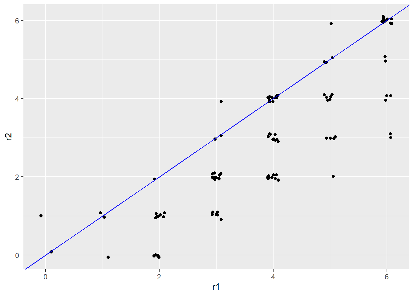

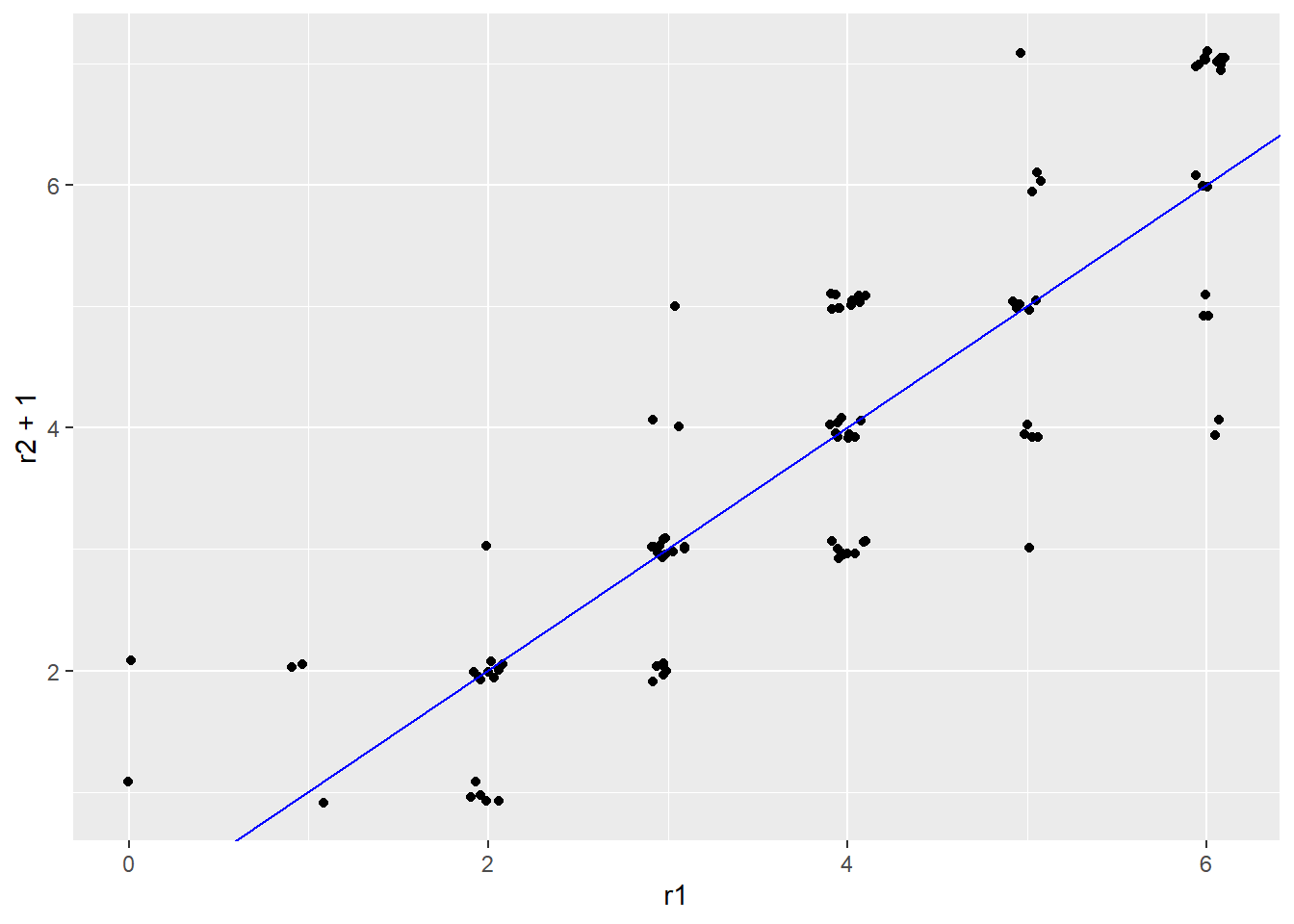
Figure 13.1: Scatter plots of simulated essay scores with a systematic difference around 0.5 points.

Is it a problem that the correlation ignores systematic score differences? Can you think of any real-life situations where it wouldn’t be cause for concern? A simple example is when awarding scholarships or giving other types of awards or recognition. In these cases consistent rank ordering is key and systematic differences are less important because the purpose of the ranking is to identify the top candidate. There is no absolute scale on which subjects are rated. Instead, they are rated in comparison to one another. As a result, a systematic difference in ratings would technically not matter.

13.2 Summary

This module provided an overview of reliability within the frameworks of CTT, for items and test forms, for reliability study designs with multiple facets. After a general definition of reliability in terms of consistency in scores, the CTT model was introduced, and two commonly used indices of CTT reliability were discussed: correlation and coefficient alpha. Reliability was then presented as it relates to consistency of scores from raters. Inter-rater agreement indices were compared, along with the correlation coefficient.

13.2.1 Exercises

Use the R object scores to find the average variability in x1 for a given value on t. How does this compare to the SEM?
Use PISA09 to calculate split-half reliabilities with different combinations of reading items in each half. Then, use these in the Spearman-Brown formula to estimate reliabilities for the full-length test. Why do the results differ?
Suppose you want to reduce the SEM for a final exam in a course you are teaching. Identify three sources of measurement error that could contribute to the SEM, and three that could not. Then, consider strategies for reducing error from these sources.
Estimate the internal consistency reliability for the attitude toward school scale. Remember to reverse code items as needed.
Dr. Phil is developing a measure of relationship quality to be used in counseling settings with couples. He intends to administer the measure to couples multiple times over a series of counseling sessions. Describe an appropriate study design for examining the reliability of this measure.
More and more TV shows lately seem to involve people performing some talent on stage and then being critiqued by a panel of judges, one of whom is British. Describe the ``true score’’ for a performer in this scenario, and identify sources of measurement error that could result from the judging process, including both systematic and random sources of error.
With proportion agreement, consider the following questions. When would we expect to see 0% or nearly 0% agreement, if ever? What would the counts in the table look like if there were 0% agreement? When would we expect to see 100% or nearly 100% agreement, if ever? What would the counts in the table look like if there were 100% agreement?
What is the maximum possible value for kappa? And what would we expect the minimum possible value to be?
Given the strengths and limitations of correlation as a measure of interrater reliability, with what type of score referencing is this measure of reliability most appropriate?
Compare the interrater agreement indices with interrater reliability based on Pearson correlation. What makes the correlation coefficient useful with interval data? What does it tell us, or what does it do, that an agreement index does not?