32 IRT versus CTT

Since its development in the 1950s and 1960s (Lord 1952; Rasch 1960), IRT has become the preferred statistical methodology for item analysis and test development. The success of IRT over its predecessor CTT comes primarily from the focus in IRT on the individual components that make up a test, that is, the items themselves. By modeling outcomes at the item level, rather than at the test level as in CTT, IRT is more complex but also more comprehensive in terms of the information it provides about test performance.

32.1 CTT review

As discussed previously, CTT gives us a model for the observed total score \(X\). This model decomposes \(X\) into two parts, truth \(T\) and error \(E\):

\[\begin{equation} X = T + E. \end{equation}\]

The true score \(T\) is the construct we’re intending to measure, and we assume it plays some systematic role in causing people to obtain observed scores on \(X\). The error \(E\) is everything randomly unrelated to the construct we’re intending to measure. Error also has a direct impact on \(X\). From Module 26, two item statistics that come from CTT are the mean performance on a given item, referred to as the \(p\)-value for dichotomous items, and the (corrected) item-total correlation for an item. Before moving on, you should be familiar with these two statistics, item difficulty and item discrimination, how they are related, and what they tell us about the items in a test.

It should be apparent that CTT is a relatively simple model of test performance. The simplicity of the model brings up its main limitation: the score scale is dependent on the items in the test and the people taking the test. The results of CTT are said to be sample dependent because 1) any \(X\), \(T\), or \(E\) that you obtain for a particular test taker only has meaning within the test she or he took, and 2) any item difficulty or discrimination statistics you estimate only have meaning within a particular sample of test takers. So, the person parameters are dependent on the test we use, and the item parameters are dependent on the test takers.

For example, suppose an instructor gives the same final exam to a new classroom of students each semester. At the first administration, the CITC discrimination for one item is 0.08. That’s low, and it suggests that there’s a problem with the item. However, in the second administration of the same exam to another group of students, the same item is found to have a CITC of 0.52. Which of these discriminations is correct? According to CTT, they’re both correct, for the sample with which they are calculated. In CTT there is technically no absolute item difficulty or discrimination that generalizes across samples or populations of examinees. The same goes for ability estimates. If two students take different final exams for the same course, each with different items but the same number of items, ability estimates will depend on the difficulty and quality of the respective exams. There is no absolute ability estimate that generalizes across samples of items. This is the main limitation of CTT: parameters that come from the model are sample and test dependent.

A second major limitation of CTT results from the fact that the model is specified using total scores. Because we rely on total scores in CTT, a given test only produces one estimate of reliability and, thus, one estimate of SEM, and these are assumed to be unchanging for all people taking the test. The measurement error we expect to see in scores would be the same regardless of level on the construct. This limitation is especially problematic when test items do not match the ability level of a particular group of people. For example, consider a comprehensive vocabulary test covering all of the words taught in a fourth grade classroom. The test is given to a group of students just starting fourth grade, and another group who just completed fourth grade and is starting fifth. Students who have had the opportunity to learn the test content should respond more reliably than students who have not. Yet, the test itself has a single reliability and SEM that would be used to estimate measurement error for any score. Thus, the second major limitation of CTT is that reliability and SEM are constant and do not depend on the construct.

32.2 Comparing with IRT

IRT addresses the limitations of CTT, the limitations of sample and test dependence and a single constant SEM. As in CTT, IRT also provides a model of test performance. However, the model is defined at the item level, meaning there is, essentially, a separate model equation for each item in the test. So, IRT involves multiple item score models, as opposed to a single total score model. When the assumptions of the model are met, IRT parameters are, in theory, sample and item independent. This means that a person should have the same ability estimate no matter which set of items she or he takes, assuming the items pertain to the same test. And in IRT, a given item should have the same difficulty and discrimination no matter who is taking the test.

IRT also takes into account the difficulty of the items that a person responds to when estimating the person’s ability or trait level. Although the construct estimate itself, in theory, does not depend on the items, the precision with which we estimate it does depend on the items taken. Estimates of the ability or trait are more precise when they’re based on items that are close to a person’s construct level. Precision decreases when there are mismatches between person construct and item difficulty. Thus, SEM in IRT can vary by the ability of the person and the characteristics of the items given.

The main limitation of IRT is that it is a complex model requiring much larger samples of people than would be needed to utilize CTT. Whereas in CTT the recommended minimum is 100 examinees for conducting an item analysis (see Module 26), in IRT, as many as 500 or 1000 examinees may be needed to obtain stable results, depending on the complexity of the chosen model.

# Prepping data for examples
# Create subset of data for Great Britain, then reduce to 
# complete data
ritems <- c("r414q02", "r414q11", "r414q06", "r414q09",
  "r452q03", "r452q04", "r452q06", "r452q07", "r458q01",
  "r458q07", "r458q04")
rsitems <- paste0(ritems, "s")
PISA09$rtotal <- rowSums(PISA09[, rsitems])
pisagbr <- PISA09[PISA09$cnt == "GBR",
  c(rsitems, "rtotal")]
pisagbr <- pisagbr[complete.cases(pisagbr), ]

Another key difference between IRT and CTT has to do with the shape of the relationship that we estimate between item score and construct score. The CTT discrimination models a simple linear relationship between the two, whereas IRT models a curvilinear relationship between them. Recall from Module 26 that the discrimination for an item can be visualized within a scatter plot, with the construct on the \(x\)-axis and item scores on the \(y\)-axis. A strong positive item discrimination would be shown by points for incorrect scores bunching up at the bottom of the scale, and points for correct scores bunching up at the top. A line passing through these points would then have a positive slope. Because they’re based on correlations, ITC and CITC discriminations are always represented by a straight line. See Figure 32.1 for an example based on PISA09 reading item r452q06s.

# Get p-values conditional on rtotal
# tapply() applies a function to the first argument over
# subsets of data defined by the second argument
pvalues <- data.frame(rtotal = 0:11,
  p = tapply(pisagbr$r452q06s, pisagbr$rtotal, mean))
# Plot CTT discrimination over scatter plot of scored item
# responses
ggplot(pisagbr, aes(rtotal, r414q06s)) +
  geom_point(position = position_jitter(w = 0.1,
    h = 0.1)) +
  geom_smooth(method = "lm", fill = NA) +
  geom_point(aes(rtotal, p), data = pvalues,
    col = "green", size = 3)
#> `geom_smooth()` using formula 'y ~ x'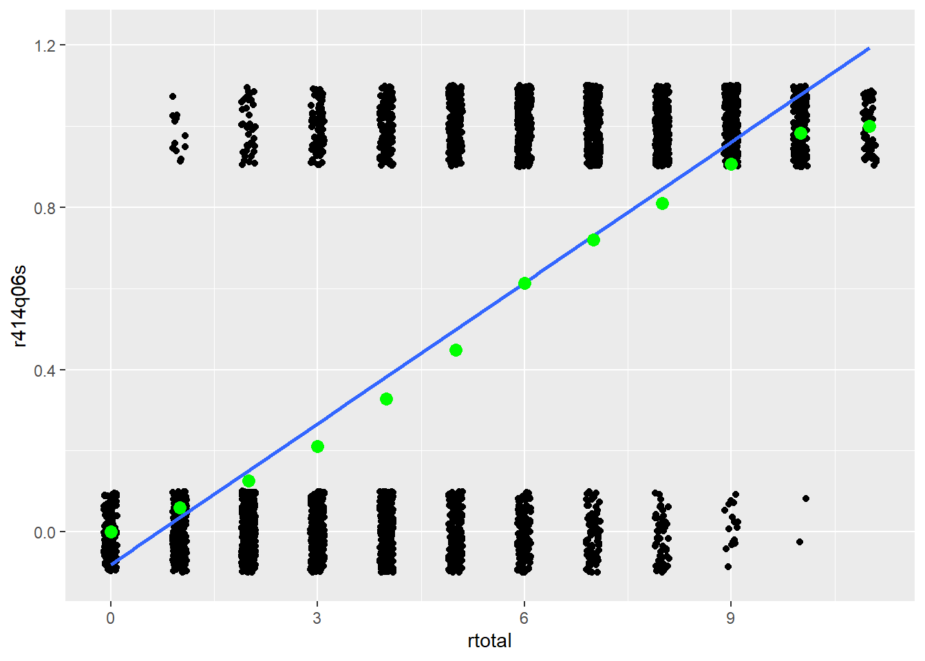

Figure 32.1: Scatter plots showing the relationship between total scores on the x-axis and scores from PISA item r452q06s on the y-axis. Lines represent the relationship between the construct and item scores for CTT (straight) and IRT (curved).

In IRT, the relationship between item and construct is similar to CTT, but the line follows what’s called a logistic curve. To demonstrate the usefulness of a logistic curve, we calculate a set of \(p\)-values for item r452q06s conditional on the construct. In Figure 32.1, the green points are \(p\)-values calculated within each group of people having the same total reading score. For example, the \(p\)-value on this item for students with a total score of 3 is about 0.20. As expected, people with lower totals have more incorrect than correct responses. As total scores increase, the number of people getting the item correct steadily increases. At a certain total score, around 5.5, we see roughly half the people get the item correct. Then, as we continue up the theta scale, more and more people get the item correct. IRT is used to capture the trend shown by the conditional \(p\)-values in Figure 32.1.