24 Confirmatory factor analysis
Confirmatory factor analysis or CFA is used to confirm an appropriate factor structure for an instrument. Whereas EFA provides tools for exploring factor structure, it does not allow us to modify specific features of our model beyond the number of factors. Furthermore, EFA does not formally support the testing of model fit or statistical significance in our results. CFA extends EFA by providing a framework for proposing a specific measurement model, fitting the model, and then testing statistically for the appropriateness or accuracy of the model given our instrument and data.
Note that CFA falls within a much broader and more general class of structural equation modeling (SEM) methods. Other applications of SEM include path analysis, multilevel regression modeling, and latent growth modeling. CFA and SEM models can be fit and analyzed in R, but, given their complexity, commercial software is often preferable, depending on the model and type of data used. For demonstration purposes, we will examine CFA in R using the lavaan package.
The BDI-II
Let’s consider again the BDI-II, discussed above in terms of EFA. Exploring the factor structure of the instrument gives us insights into the number of factors needed to adequately capture certain percentages of the variability in scores. Again, results indicate that two factors, labeled in previous studies as cognitive and somatic, account for about a quarter of the total score variance. In the plot above, these two factors clearly stand out above the scree. But the question remains, is a two factor model correct? And, if so, what is the best configuration of item loadings on those two factors?
In the end, there is no way to determine with certainty that a model is correct for a given data set and instrument. Instead, in CFA a model can be considered adequate or appropriate based on two general criteria. The first has to do with the explanatory power of the model. We might consider a model adequate when it exceeds some threshold for percentage of variability explained, and thereby minimizes in some way error variance or variability unexplained. The second criterion involves the relative appropriateness of a given model compared to other competing models. Comparisons are typically made using statistical estimates of model fit, as discussed below.
Numerous studies have employed CFA to test for the appropriateness of a two factor structure in the BDI-II. Whisman, Perez, and Ramel (2000) proposed an initial factor structure that included five BDI-II items loading on the somatic factor, and 14 items loading on the cognitive factor (the authors label this factor cognitive-affective). The remaining two items, Pessimism and Loss of Interest in Sex, had been found in exploratory analyses not to load strongly on either factor. Thus, loadings for these were not estimated in the initial CFA model.
Results for this first CFA showed poor fit. Whisman, Perez, and Ramel (2000) reported a few different fit indices, including a Comparative Fit Index (CFI) of 0.80 and a Root Mean Square Error of Approximation (RMSEA) of 0.08. Commonly used thresholds for determining “good fit” are CFI at or above 0.90 and RMSEA at or below 0.05.
An important feature of factor analysis that we have not yet discussed has to do with the relationships among item errors. In EFA, we assume that all item errors are uncorrelated. This means that the unexplained variability for a given item does not relate to the unexplained variability for any other. Similar to the CTT model, variability in EFA can only come from the estimated factors or random, uncorrelated noise. In CFA, we can relax this assumption by allowing certain error terms to correlate.
Whisman, Perez, and Ramel (2000) allowed error terms to correlate for the following pairs of items: sadness and crying, self-dislike and self-criticalness, and loss of pleasure and loss of interest. This choice to have correlated errors seems justified, given the apparent similarities in content for these items. The two factors in the initial CFA didn’t account for the fact that respondents would answer similarly within these pairs of items. Thus, the model was missing an important feature of the data.
Having allowed for correlated error terms, the two unassigned items Pessimism and Loss of Interest in Sex were also specified to load on the cognitive factor. The result was a final model with more acceptable fit statistics, including CFI of 0.90 and RMSEA of 0.06.
24.1 Steps in CFA
Here, we will fit the final model from Whisman, Perez, and Ramel (2000), while demonstrating the following basic steps in conducting a CFA:
- hypothesizing the proposed factor structure with necessary constraints,
- preparing our data and fitting the CFA model,
- evaluating the model and statistically testing for model fit,
- revising the model, comparing to more or less complex models, and repeating evaluation and testing of fit as needed.
1. Hypothesize the factor structure
As discussed previously, we hypothesize that two factors will be sufficient for explaining the correlations among items in the BDI-II. These factors are labeled cognitive and somatic, based on the content of the items that tend to load on them. We also hypothesize that the two factors will be correlated. Finally, we allow for correlated errors between sadness and crying, self-dislike and self-criticalness, and loss of pleasure and loss of interest.
Figure 24.1 is a visual representation of the CFA model we’re fitting. On the left are the two factors, and on the right are the observed item variables. Estimates for the correlation between factors, the factor loadings, and item variances are also shown.
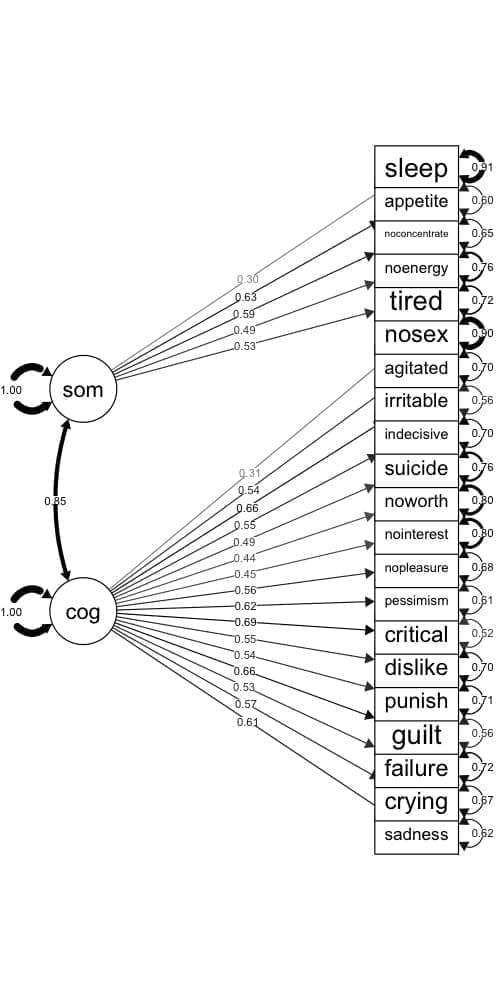
Figure 24.1: CFA model for the BDI-II, with factor loadings and error variances.
2. Prepare the data, fit the model
We assume that the scored item responses on the BDI-II represent continuous variables. The covariance matrix in BDI$S was obtained using the 576 respondents having complete data across all 21 items. As reported in Whisman, Perez, and Ramel (2000), the mean total score was 8.36 with SD 7.16. Thus, on average, respondents were in the minimal depression score range, though some had scores in the mild and moderate ranges, and a few fell in the severe range.
Considering the complexity of our model, the sample size of 576 should be sufficient for estimation purposes. Since different CFA models can involve different numbers of estimated parameters for the same number of items, sample size guidelines are usually stated in terms of the number of parameters rather than the number of items. We’ll consider the recommended minimum of five times as many people as parameters. The total number of parameters estimated by our model will be 43, with 21 factor loadings, 21 error variances, and the correlation between the cognitive and somatic factors.
We fit our CFA using the covariance matrix in BDI$S. The cfa() function in the lavaan package requires that we name each factor and then list out the items that load on it after the symbol =~. Here, we label our cognitive factor cog and somatic factor som. The items listed after each factor must match the row or column names in the covariance matrix, and must be separated by +.
The lavaanify() function will automatically add error variances for each item, and the correlation between factors, so we don’t have to write those out. We do need to add the three correlated error terms, for example, with sadness ~~ crying, where the ~~ indicates that the variable on the left covaries with the one on the right.
The model is fit using the cfa() function. We supply the model specification object that we created above, along with the covariance matrix and sample size.
# CFA of BDI using the lavaan package
# Specify the factor structure
# Comments within the model statement are ignored
bdimod <- lavaanify(model = "
  # Latent variable definitions
  cog =~ sadness + crying + failure + guilt + punish +
    dislike + critical + pessimism + nopleasure +
    nointerest + noworth + suicide + indecisive +
    irritable + agitated + nosex
  som =~ tired + noenergy + noconcentrate + appetite +
    sleep
  # Covariances
  sadness ~~ crying
  dislike ~~ critical
  nopleasure ~~ nointerest",
  auto.var = TRUE, auto.cov.lv.x = TRUE, std.lv = TRUE)
# Fit the model
bdicfa <- cfa(bdimod, sample.cov = BDI$S,
  sample.nobs = 576)
3. Evaluate the model
To evaluate the model that’s stored in the object bdicfa, we send it to the lavaan summary() function, while requesting fit indices with the argument fit = TRUE. Lots of output are printed to the console, including a summary of the model estimation, some fit statistics, factor loadings (under Latent Variables), covariances, and variance terms (including item errors).
The CFI and RMSEA are printed in the top half of the output. Neither statistic reaches the threshold we’d hope for. CFI is 0.84 and RMSEA is 0.07, indicating less than optimal fit.
Standardized factor loadings are shown in the last column of the Latent Variables output. Some of the loadings match up well with those reported in the original study. Others are different. The discrepancies may be due to the fact that our CFA was run on correlations rounded to two decimal places that were converted using standard deviations to covariances, whereas raw data were used in the original study. Rounding can result in a loss of meaningful information.
# Print fit indices, loadings, and other output
summary(bdicfa, fit = TRUE, standardized = TRUE)
#> lavaan 0.6-9 ended normally after 41 iterations
#>
#>   Estimator                                         ML
#>   Optimization method                           NLMINB
#>   Number of model parameters                        46
#>
#>   Number of observations                           576
#>
#> Model Test User Model:
#>
#>   Test statistic                               737.735
#>   Degrees of freedom                               185
#>   P-value (Chi-square)                           0.000
#>
#> Model Test Baseline Model:
#>
#>   Test statistic                              3666.723
#>   Degrees of freedom                               210
#>   P-value                                        0.000
#>
#> User Model versus Baseline Model:
#>
#>   Comparative Fit Index (CFI)                    0.840
#>   Tucker-Lewis Index (TLI)                       0.818
#>
#> Loglikelihood and Information Criteria:
#>
#>   Loglikelihood user model (H0)              -9585.792
#>   Loglikelihood unrestricted model (H1)      -9216.925
#>
#>   Akaike (AIC)                               19263.585
#>   Bayesian (BIC)                             19463.966
#>   Sample-size adjusted Bayesian (BIC)        19317.934
#>
#> Root Mean Square Error of Approximation:
#>
#>   RMSEA                                          0.072
#>   90 Percent confidence interval - lower         0.067
#>   90 Percent confidence interval - upper         0.078
#>   P-value RMSEA <= 0.05                          0.000
#>
#> Standardized Root Mean Square Residual:
#>
#>   SRMR                                           0.057
#>
#> Parameter Estimates:
#>
#>   Standard errors                             Standard
#>   Information                                 Expected
#>   Information saturated (h1) model          Structured
#>
#> Latent Variables:
#>                    Estimate  Std.Err  z-value  P(>|z|)   Std.lv  Std.all
#>   cog =~
#>     sadness           0.349    0.022   15.515    0.000    0.349    0.613
#>     crying            0.315    0.022   14.267    0.000    0.315    0.572
#>     failure           0.314    0.024   13.140    0.000    0.314    0.533
#>     guilt             0.391    0.023   17.222    0.000    0.391    0.663
#>     punish            0.329    0.025   13.339    0.000    0.329    0.540
#>     dislike           0.290    0.022   13.462    0.000    0.290    0.547
#>     critical          0.472    0.026   18.233    0.000    0.472    0.695
#>     pessimism         0.412    0.026   15.935    0.000    0.412    0.624
#>     nopleasure        0.225    0.016   14.012    0.000    0.225    0.563
#>     nointerest        0.373    0.035   10.795    0.000    0.373    0.450
#>     noworth           0.261    0.025   10.637    0.000    0.261    0.443
#>     suicide           0.268    0.023   11.859    0.000    0.268    0.488
#>     indecisive        0.358    0.026   13.661    0.000    0.358    0.551
#>     irritable         0.390    0.023   17.179    0.000    0.390    0.662
#>     agitated          0.327    0.024   13.494    0.000    0.327    0.545
#>     nosex             0.225    0.031    7.200    0.000    0.225    0.309
#>   som =~
#>     tired             0.295    0.024   12.048    0.000    0.295    0.527
#>     noenergy          0.375    0.033   11.202    0.000    0.375    0.494
#>     noconcentrate     0.425    0.031   13.748    0.000    0.425    0.591
#>     appetite          0.391    0.026   14.825    0.000    0.391    0.630
#>     sleep             0.137    0.021    6.523    0.000    0.137    0.299
#>
#> Covariances:
#>                    Estimate  Std.Err  z-value  P(>|z|)   Std.lv  Std.all
#>  .sadness ~~
#>    .crying            0.009    0.009    1.007    0.314    0.009    0.045
#>  .dislike ~~
#>    .critical         -0.029    0.010   -2.919    0.004   -0.029   -0.133
#>  .nopleasure ~~
#>    .nointerest        0.039    0.011    3.572    0.000    0.039    0.158
#>   cog ~~
#>     som               0.847    0.028   30.370    0.000    0.847    0.847
#>
#> Variances:
#>                    Estimate  Std.Err  z-value  P(>|z|)   Std.lv  Std.all
#>    .sadness           0.203    0.013   15.727    0.000    0.203    0.625
#>    .crying            0.203    0.013   15.948    0.000    0.203    0.672
#>    .failure           0.249    0.015   16.193    0.000    0.249    0.716
#>    .guilt             0.195    0.013   15.424    0.000    0.195    0.560
#>    .punish            0.263    0.016   16.165    0.000    0.263    0.709
#>    .dislike           0.196    0.012   16.006    0.000    0.196    0.700
#>    .critical          0.239    0.016   14.991    0.000    0.239    0.517
#>    .pessimism         0.265    0.017   15.715    0.000    0.265    0.610
#>    .nopleasure        0.109    0.007   16.043    0.000    0.109    0.683
#>    .nointerest        0.549    0.033   16.451    0.000    0.549    0.798
#>    .noworth           0.279    0.017   16.492    0.000    0.279    0.804
#>    .suicide           0.230    0.014   16.359    0.000    0.230    0.762
#>    .indecisive        0.294    0.018   16.117    0.000    0.294    0.697
#>    .irritable         0.195    0.013   15.435    0.000    0.195    0.562
#>    .agitated          0.253    0.016   16.142    0.000    0.253    0.703
#>    .nosex             0.481    0.029   16.764    0.000    0.481    0.905
#>    .tired             0.226    0.015   15.157    0.000    0.226    0.723
#>    .noenergy          0.436    0.028   15.458    0.000    0.436    0.756
#>    .noconcentrate     0.337    0.023   14.387    0.000    0.337    0.651
#>    .appetite          0.231    0.017   13.737    0.000    0.231    0.603
#>    .sleep             0.192    0.012   16.521    0.000    0.192    0.911
#>     cog               1.000                               1.000    1.000
#>     som               1.000                               1.000    1.000
4. Revise as needed
The discouraging CFA results may inspire us to modify our factor structure in hopes of improving model fit. Potential changes include the removal of items with low factor loadings, the correlating of more or fewer error terms, and the evaluation of different numbers of factors. Having fit multiple CFA models, we can then compare fit indices and look for relative improvements in fit for one model over another.
Let’s quickly examine a CFA where all items load on a single factor. We no longer have correlated error terms, and item errors are again added automatically. We only specify the loading of all items on our single factor, labeled depression.
# Specify the factor structure
# Comments within the model statement are ignored as
# comments
bdimod2 <- lavaanify(model = "
  depression =~ sadness + crying + failure + guilt +
    punish + dislike + critical + pessimism + nopleasure +
    nointerest + noworth + suicide + indecisive +
    irritable + agitated + nosex + tired + noenergy +
    noconcentrate + appetite + sleep",
  auto.var = TRUE, std.lv = TRUE)
# Fit the model
bdicfa2 <- cfa(bdimod2, sample.cov = BDI$S,
  sample.nobs = 576)
# Print output
summary(bdicfa2, fit = TRUE, standardized = TRUE)
#> lavaan 0.6-9 ended normally after 29 iterations
#>
#>   Estimator                                         ML
#>   Optimization method                           NLMINB
#>   Number of model parameters                        42
#>
#>   Number of observations                           576
#>
#> Model Test User Model:
#>
#>   Test statistic                               792.338
#>   Degrees of freedom                               189
#>   P-value (Chi-square)                           0.000
#>
#> Model Test Baseline Model:
#>
#>   Test statistic                              3666.723
#>   Degrees of freedom                               210
#>   P-value                                        0.000
#>
#> User Model versus Baseline Model:
#>
#>   Comparative Fit Index (CFI)                    0.825
#>   Tucker-Lewis Index (TLI)                       0.806
#>
#> Loglikelihood and Information Criteria:
#>
#>   Loglikelihood user model (H0)              -9613.094
#>   Loglikelihood unrestricted model (H1)      -9216.925
#>
#>   Akaike (AIC)                               19310.188
#>   Bayesian (BIC)                             19493.144
#>   Sample-size adjusted Bayesian (BIC)        19359.811
#>
#> Root Mean Square Error of Approximation:
#>
#>   RMSEA                                          0.074
#>   90 Percent confidence interval - lower         0.069
#>   90 Percent confidence interval - upper         0.080
#>   P-value RMSEA <= 0.05                          0.000
#>
#> Standardized Root Mean Square Residual:
#>
#>   SRMR                                           0.058
#>
#> Parameter Estimates:
#>
#>   Standard errors                             Standard
#>   Information                                 Expected
#>   Information saturated (h1) model          Structured
#>
#> Latent Variables:
#>                    Estimate  Std.Err  z-value  P(>|z|)   Std.lv  Std.all
#>   depression =~
#>     sadness           0.352    0.022   15.780    0.000    0.352    0.619
#>     crying            0.313    0.022   14.230    0.000    0.313    0.569
#>     failure           0.305    0.024   12.736    0.000    0.305    0.518
#>     guilt             0.394    0.023   17.432    0.000    0.394    0.669
#>     punish            0.322    0.025   13.059    0.000    0.322    0.529
#>     dislike           0.281    0.021   13.082    0.000    0.281    0.530
#>     critical          0.462    0.026   17.798    0.000    0.462    0.679
#>     pessimism         0.407    0.026   15.751    0.000    0.407    0.618
#>     nopleasure        0.224    0.016   13.974    0.000    0.224    0.560
#>     nointerest        0.381    0.034   11.106    0.000    0.381    0.460
#>     noworth           0.264    0.024   10.781    0.000    0.264    0.448
#>     suicide           0.270    0.023   11.999    0.000    0.270    0.492
#>     indecisive        0.361    0.026   13.843    0.000    0.361    0.556
#>     irritable         0.384    0.023   16.846    0.000    0.384    0.651
#>     agitated          0.335    0.024   13.954    0.000    0.335    0.560
#>     nosex             0.234    0.031    7.520    0.000    0.234    0.321
#>     tired             0.279    0.023   12.174    0.000    0.279    0.498
#>     noenergy          0.329    0.032   10.391    0.000    0.329    0.433
#>     noconcentrate     0.374    0.029   12.789    0.000    0.374    0.520
#>     appetite          0.331    0.025   13.192    0.000    0.331    0.534
#>     sleep             0.138    0.020    7.013    0.000    0.138    0.301
#>
#> Variances:
#>                    Estimate  Std.Err  z-value  P(>|z|)   Std.lv  Std.all
#>    .sadness           0.200    0.013   15.800    0.000    0.200    0.617
#>    .crying            0.204    0.013   16.068    0.000    0.204    0.677
#>    .failure           0.254    0.016   16.279    0.000    0.254    0.732
#>    .guilt             0.192    0.012   15.442    0.000    0.192    0.553
#>    .punish            0.267    0.016   16.237    0.000    0.267    0.720
#>    .dislike           0.202    0.012   16.234    0.000    0.202    0.719
#>    .critical          0.249    0.016   15.351    0.000    0.249    0.539
#>    .pessimism         0.269    0.017   15.805    0.000    0.269    0.618
#>    .nopleasure        0.110    0.007   16.107    0.000    0.110    0.686
#>    .nointerest        0.542    0.033   16.466    0.000    0.542    0.789
#>    .noworth           0.278    0.017   16.498    0.000    0.278    0.800
#>    .suicide           0.229    0.014   16.368    0.000    0.229    0.758
#>    .indecisive        0.291    0.018   16.127    0.000    0.291    0.691
#>    .irritable         0.200    0.013   15.579    0.000    0.200    0.576
#>    .agitated          0.247    0.015   16.110    0.000    0.247    0.687
#>    .nosex             0.477    0.028   16.754    0.000    0.477    0.897
#>    .tired             0.235    0.014   16.348    0.000    0.235    0.752
#>    .noenergy          0.468    0.028   16.535    0.000    0.468    0.813
#>    .noconcentrate     0.378    0.023   16.272    0.000    0.378    0.730
#>    .appetite          0.274    0.017   16.219    0.000    0.274    0.715
#>    .sleep             0.192    0.011   16.783    0.000    0.192    0.910
#>     depression        1.000                               1.000    1.000
We can compare fit indices for our two models using the anova() function. This comparison requires that the same data be used to fit all the models of interest. So, it wouldn’t be appropriate to compare bdimod with another model fit to only 20 of the 21 BDI-II items.
Three comparison statistics are provided by anova(). With Akaike’s Information Criterion (AIC) and the Bayesian Information Criterion (BIC), we’re looking for the model with the smallest value. Smaller AIC and smaller BIC from one model to the next indicate better fit. The chi-square statistic has a p-value associated with it, where a p-value below a certain cutoff such as 0.05 would indicate significantly better fit for one model over another.
# Compare fit for BDI CFA models
anova(bdicfa2, bdicfa)
#> Chi-Squared Difference Test
#>
#>          Df   AIC   BIC Chisq Chisq diff Df diff Pr(>Chisq)
#> bdicfa  185 19264 19464   738
#> bdicfa2 189 19310 19493   792       54.6       4    3.9e-11 ***
#> ---
#> Signif. codes:  0 '***' 0.001 '**' 0.01 '*' 0.05 '.' 0.1 ' ' 1
Of these three fit comparison statistics, we will focus on AIC and BIC. The AIC and BIC both increase from the model with two factors to the model with only one. This indicates poorer model fit for the depression model.
Overall, results for the unidimensional model are no better than for the previous one. The AIC and BIC are both larger, and the CFI and RMSEA are relatively unchanged. Most loadings are moderately positive, but some leave a substantial amount of item variability unexplained. For example, the item error terms (in the Std.all column of the Variances table) for sleep and noenergy are both larger than 0.80. These results indicate that more than 80% of the variability is unexplained for these items. Errors for the remaining items are all above 0.50.
Taken together, the results of these CFA suggest that the two-factor and unidimensional models may not be appropriate for the BDI-II, at least in the undergraduate population with which the data were collected.
24.2 Confirming PISA Approaches to Learning
In our final demonstration, we’ll fit a CFA to the PISA Approaches to Learning items. Our first factor structure is similar to what we explored previously via EFA. However, here, our items are only allowed to load on their intended factors. We’re hypothesizing that any cross loadings on other factors are negligible and not essential to the underlying factor structure for the instrument.
# CFA with PISA approaches to learning scale
# Specify the factor structure
almod <- lavaanify(model = "
  # Three factors
  memor =~ st27q01 + st27q03 + st27q05 + st27q07
  elab =~ st27q04 + st27q08 + st27q10 + st27q12
  cstrat =~ st27q02 + st27q06 + st27q09 + st27q11 +
    st27q13",
  auto.var = TRUE, auto.cov.lv.x = TRUE, std.lv = TRUE)
# Fit the model
alcfa <- cfa(almod, sample.cov = cov(pisagbr[, alitems]),
  sample.nobs = 3514)
# Print output
summary(alcfa, fit = TRUE, standardized = TRUE)
#> lavaan 0.6-9 ended normally after 20 iterations
#>
#>   Estimator                                         ML
#>   Optimization method                           NLMINB
#>   Number of model parameters                        29
#>
#>   Number of observations                          3514
#>
#> Model Test User Model:
#>
#>   Test statistic                              1474.664
#>   Degrees of freedom                                62
#>   P-value (Chi-square)                           0.000
#>
#> Model Test Baseline Model:
#>
#>   Test statistic                             12390.734
#>   Degrees of freedom                                78
#>   P-value                                        0.000
#>
#> User Model versus Baseline Model:
#>
#>   Comparative Fit Index (CFI)                    0.885
#>   Tucker-Lewis Index (TLI)                       0.856
#>
#> Loglikelihood and Information Criteria:
#>
#>   Loglikelihood user model (H0)             -52923.964
#>   Loglikelihood unrestricted model (H1)     -52186.632
#>
#>   Akaike (AIC)                              105905.928
#>   Bayesian (BIC)                            106084.699
#>   Sample-size adjusted Bayesian (BIC)       105992.552
#>
#> Root Mean Square Error of Approximation:
#>
#>   RMSEA                                          0.081
#>   90 Percent confidence interval - lower         0.077
#>   90 Percent confidence interval - upper         0.084
#>   P-value RMSEA <= 0.05                          0.000
#>
#> Standardized Root Mean Square Residual:
#>
#>   SRMR                                           0.057
#>
#> Parameter Estimates:
#>
#>   Standard errors                             Standard
#>   Information                                 Expected
#>   Information saturated (h1) model          Structured
#>
#> Latent Variables:
#>                    Estimate  Std.Err  z-value  P(>|z|)   Std.lv  Std.all
#>   memor =~
#>     st27q01           0.476    0.015   32.615    0.000    0.476    0.585
#>     st27q03           0.509    0.014   36.402    0.000    0.509    0.644
#>     st27q05           0.541    0.016   33.380    0.000    0.541    0.597
#>     st27q07           0.556    0.017   33.656    0.000    0.556    0.601
#>   elab =~
#>     st27q04           0.470    0.016   30.098    0.000    0.470    0.534
#>     st27q08           0.577    0.015   37.460    0.000    0.577    0.644
#>     st27q10           0.650    0.016   41.722    0.000    0.650    0.706
#>     st27q12           0.660    0.015   43.070    0.000    0.660    0.725
#>   cstrat =~
#>     st27q02           0.460    0.014   31.931    0.000    0.460    0.550
#>     st27q06           0.562    0.014   39.938    0.000    0.562    0.662
#>     st27q09           0.547    0.014   39.525    0.000    0.547    0.657
#>     st27q11           0.544    0.013   40.705    0.000    0.544    0.672
#>     st27q13           0.551    0.016   34.522    0.000    0.551    0.588
#>
#> Covariances:
#>                    Estimate  Std.Err  z-value  P(>|z|)   Std.lv  Std.all
#>   memor ~~
#>     elab              0.368    0.021   17.565    0.000    0.368    0.368
#>     cstrat            0.714    0.015   46.863    0.000    0.714    0.714
#>   elab ~~
#>     cstrat            0.576    0.017   34.248    0.000    0.576    0.576
#>
#> Variances:
#>                    Estimate  Std.Err  z-value  P(>|z|)   Std.lv  Std.all
#>    .st27q01           0.435    0.013   34.471    0.000    0.435    0.658
#>    .st27q03           0.365    0.012   31.715    0.000    0.365    0.585
#>    .st27q05           0.527    0.016   33.981    0.000    0.527    0.643
#>    .st27q07           0.546    0.016   33.797    0.000    0.546    0.638
#>    .st27q04           0.555    0.015   37.116    0.000    0.555    0.715
#>    .st27q08           0.471    0.014   33.242    0.000    0.471    0.586
#>    .st27q10           0.427    0.014   29.620    0.000    0.427    0.502
#>    .st27q12           0.393    0.014   28.195    0.000    0.393    0.474
#>    .st27q02           0.487    0.013   37.590    0.000    0.487    0.697
#>    .st27q06           0.405    0.012   34.078    0.000    0.405    0.562
#>    .st27q09           0.395    0.012   34.310    0.000    0.395    0.569
#>    .st27q11           0.359    0.011   33.630    0.000    0.359    0.548
#>    .st27q13           0.576    0.016   36.648    0.000    0.576    0.655
#>     memor             1.000                               1.000    1.000
#>     elab              1.000                               1.000    1.000
#>     cstrat            1.000                               1.000    1.000
Model fit is not as impressive as we would hope. The CFI is 0.71 and the RMSEA is 0.13. As with the BDI-II, loadings are moderately positive, but they leave the majority of the item variance unexplained. These results suggest that the Approaches to Learning constructs may not be strong enough or distinct enough to warrant the calculation of scale scores across the memorization, elaboration, and control items.