11 Statistical definition of reliability.
In CTT, reliability is defined as the proportion of variability in \(X\) that is due to variability in true scores \(T\):
\[\begin{equation} r = \frac{\sigma^2_T}{\sigma^2_X}. \tag{11.1} \end{equation}\]
11.1 Estimating reliability
One indirect estimate made possible by CTT is the correlation between scores on two forms of the same test:
\[\begin{equation} r = \rho_{X_1 X_2} = \frac{\sigma_{X_1 X_2}}{\sigma_{X_1} \sigma_{X_2}}. \tag{11.2} \end{equation}\]
11.2 Split-half method
The split-half method takes scores on a single test form, and separates them into scores on two halves of the test, which are treated as separate test forms. The correlation between these two halves then represents an indirect estimate of reliability, based on Equation (11.1).
# Split half correlation, assuming we only had scores on
# one test form
# With an odd number of reading items, one half has 5
# items and the other has 6
library(epmr)

xsplit1 <- rowSums(PISA09[PISA09$cnt == "BEL",
  rsitems[1:5]])
xsplit2 <- rowSums(PISA09[PISA09$cnt == "BEL",
  rsitems[6:11]])

cor(xsplit1, xsplit2, use = "complete")
#> [1] 0.625
11.3 Spearman Brown
The Spearman-Brown formula was originally used to correct for the reduction in reliability that occurred when correlating two test forms that were only half the length of the original test. In theory, reliability will increase as we add items to a test. Thus, Spearman-Brown is used to estimate, or predict, what the reliability would be if the half-length tests were made into full-length tests.
# sb_r() in the epmr package uses the Spearman-Brown
# formula to estimate how reliability would change when
# test length changes by a factor k
# If test length were doubled, k would be 2
sb_r(r = cor(xsplit1, xsplit2, use = "complete"), k = 2)
#> [1] 0.769
The Spearman-Brown reliability, \(r_{new}\), is estimated as a function of what’s labeled here as the old reliability, \(r_{old}\), and the factor by which the length of \(X\) is predicted to change, \(k\):
\[\begin{equation} r_{new} = \frac{kr_{old}}{(k - 1)r_{old} + 1}. \tag{11.3} \end{equation}\]
Again, \(k\) is the factor by which the test length is increased or decreased. It is equal to the number of items in the new test divided by the number of items in the original test. Multiply \(k\) by the old reliability, and then divided the result by \((k - 1)\) times the old reliability, plus 1. The epmr package contains sb_r(), a simple function for estimating the Spearman-Brown reliability.
11.4 Standard Error of Measurement
Typically, we’re more interested in how the unreliability of a test can be expressed in terms of the available observed variability. Thus, we multiply the unreliable proportion of variance by the standard deviation of \(X\) to obtain the SEM:
\[\begin{equation} SEM = \sigma_X\sqrt{1 - r}. \tag{11.4} \end{equation}\]
Confidence intervals for PISA09 can be estimated in the same way. First, we choose a measure of reliability, find the SD of observed scores, and obtain the corresponding SEM. Then, we can find the CI, which gives us the expected amount of uncertainty in our observed scores due to random measurement error. Here, we’re calculating SEM and the CI using alpha, but other reliability estimates would work as well. Figure 11.1 shows the 11 possible PISA09 reading scores in order, with error bars based on SEM for students in Belgium.
# Get alpha and SEM for students in Belgium

bela <- coef_alpha(PISA09[PISA09$cnt == "BEL", rsitems])
bela_alpha=bela$alpha
# The sem function from epmr also overlaps with sem from
# another package so we're spelling it out here in long
# form
belsem <- epmr::sem(r = bela_alpha, sd = sd(scores$x1,
  na.rm = TRUE))
# Plot the 11 possible total scores against themselves
# Error bars are shown for 1 SEM, giving a 68% confidence
# interval and 2 SEM, giving the 95% confidence interval
# x is converted to factor to show discrete values on the
# x-axis
beldat <- data.frame(x = 1:11, sem = belsem)
ggplot(beldat, aes(factor(x), x)) +
  geom_errorbar(aes(ymin = x - sem * 2,
    ymax = x + sem * 2), col = "violet") +
  geom_errorbar(aes(ymin = x - sem, ymax = x + sem),
    col = "yellow") +
  geom_point()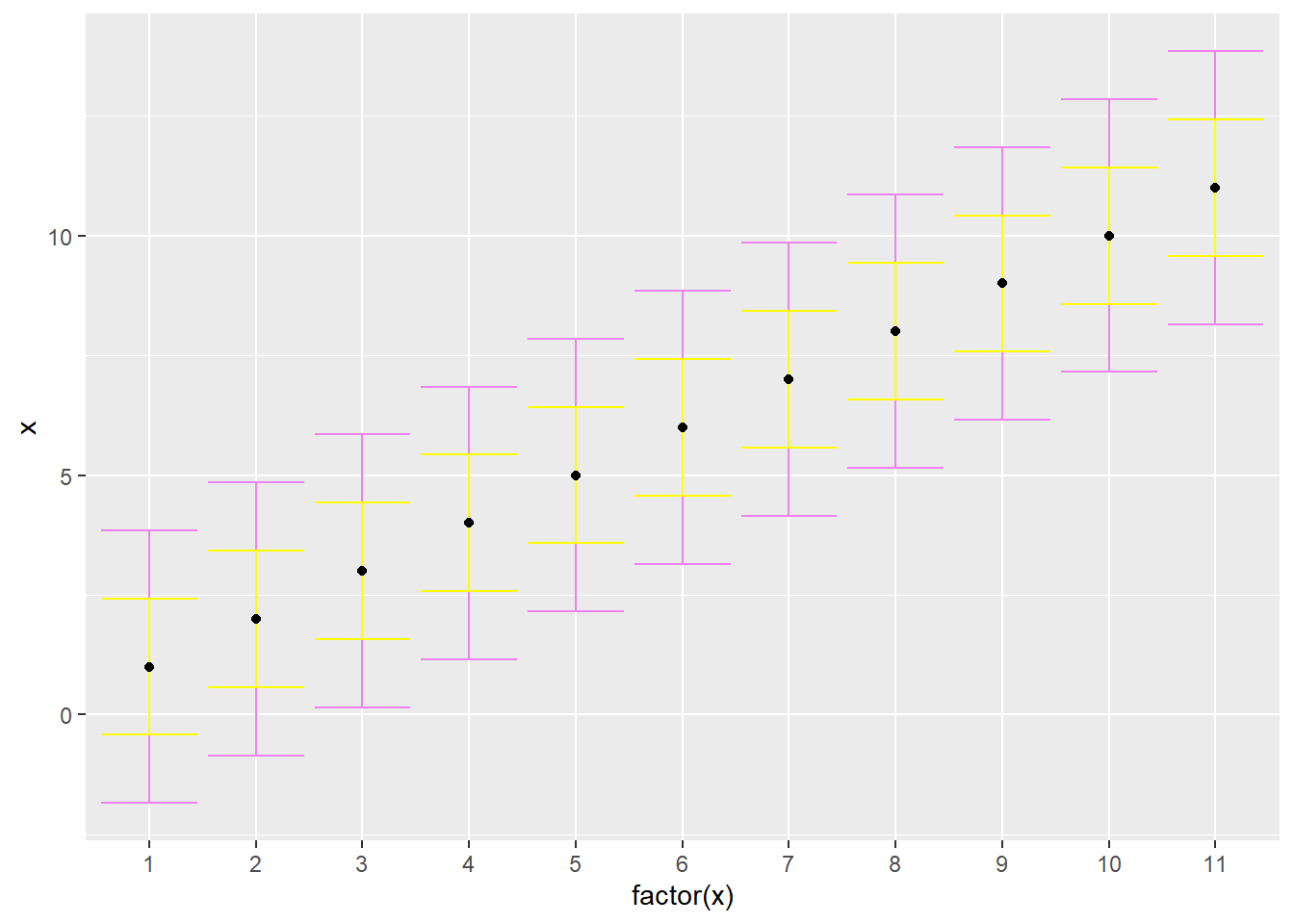
Figure 11.1: The PISA09 reading scale shown with 68 and 95 percent confidence intervals around each point.
Figure 11.1 helps us visualize the impact of unreliable measurement on score comparisons. For example, note that the top of the 95% confidence interval for \(X\) of 2 extends nearly to 5 points, and thus overlaps with the CI for adjacent scores 3 through 7. It isn’t until \(X\) of 8 that the CI no longer overlap. With a CI of belsem 1.425, we’re 95% confident that students with observed scores differing at least by belsem * 4 5.7 have different true scores. Students with observed scores closer than belsem * 4 may actually have the same true scores.