34 Applications
34.1 In practice…
As is true when comparing other statistical models, the choice of Rasch, 1PL, 2PL, or 3PL should be based on considerations of theory, model assumptions, and sample size.
Because of its simplicity and lower sample size requirements, the Rasch model is commonly used in small-scale achievement and aptitude testing, for example, with assessments developed and used at the district level, or instruments designed for use in research or lower-stakes decision-making. The IGDI measures discussed in Module ?? are developed using the Rasch model. The MAP tests, published by Northwest Evaluation Association, are also based on a Rasch model. Some consider the Rasch model most appropriate for theoretical reasons. In this case, it is argued that we should seek to develop tests that have items that discriminate equally well; items that differ in discrimination should be replaced with ones that do not. Others utilize the Rasch model as a simplified IRT model, where the sample size needed to accurately estimate different item discriminations and lower asymptotes cannot be obtained. Either way, when using the Rasch model, we should be confident in our assumption that differences between items in discrimination and lower asymptote are negligible.
The 2PL and 3PL models are often used in larger-scale testing situations, for example, on high-stakes tests such as the GRE and ACT. The large samples available with these tests support the additional estimation required by these models. And proponents of the two-parameter and three-parameter models often argue that it is unreasonable to assume zero lower asymptote, or equal discriminations across items.
In terms of the properties of the model itself, as mentioned above, IRT overcomes the CTT limitation of sample and item dependence. As a result, ability estimates from an IRT model should not depend on the sample of items used to estimate ability, and item parameter estimates should not depend on the sample of people used to estimate them. An explanation of how this is possible is beyond the scope of this book. Instead, it is important to remember that, in theory, when IRT is correctly applied, the resulting parameters are sample and item independent. As a result, they can be generalized across samples for a given population of people and test items.
IRT is useful first in item analysis, where we pilot test a set of items and then examine item difficulty and discrimination, as discussed with CTT in Module 26. The benefit of IRT over CTT is that we can accumulate difficulty and discrimination statistics for items over multiple samples of people, and they are, in theory, always expressed on the same scale. So, our item analysis results are sample independent. This is especially useful for tests that are maintained across more than one administration. Many admissions tests, for example, have been in use for decades. State tests, as another example, must also maintain comparable item statistics from year to year, since new groups of students take the tests each year.
Item banking refers to the process of storing items for use in future, potentially undeveloped, forms of a test. Because IRT allows us to estimate sample independent item parameters, we can estimate parameters for certain items using pilot data, that is, before the items are used operationally. This is what happens in a computer adaptive test. For example, the difficulty of a bank of items is known, typically from pilot administrations. When you sit down to take the test, an item of known average difficulty can then be administered. If you get the item correct, you are given a more difficult item. The process continues, with the difficulty of the items adapting based on your performance, until the computer is confident it has identified your ability level. In this way, computer adaptive testing relies heavily on IRT.
34.2 Examples
The epmr package contains functions for estimating and manipulating results from the Rasch model. Other R packages are available for estimating the 2PL and 3PL (e.g., Rizopoulos 2006). Commercial software packages are also available, and are often used when IRT is applied operationally.
Here, we estimate the Rasch model for PISA09 students in Great Britain. The data set was created at the beginning of the module. The irtstudy() function in epmr runs the Rasch model and prints some summary results, including model fit indices and variability estimates for random effect. Note that the model is being fit as a generalized linear model with random person and random item effects, using the lme4 package (Bates et al. 2015). The estimation process won’t be discussed here. For details, see Doran et al. (2007) and De Boeck et al. (2011).
# The irtstudy() function estimates theta and b parameters
# for a set of scored item responses
irtgbr <- irtstudy(pisagbr[, rsitems])
irtgbr
#>
#> Item Response Theory Study
#>
#> 3650 people, 11 items
#>
#> Model fit with lme4::glmer
#>         AIC         BIC      logLik    deviance df.residual
#>       46615       46632      -23306       38746       40148
#>
#> Random effects
#>        Std.Dev  Var
#> person    1.29 1.66
#> item      1.01 1.02
The R object returned by irtstudy() contains a list of results. The first element in the list, irtgbr$data, contains the original data set with additional columns for the theta estimate and SEM for each person. The next element in the output list, irtgbr$ip, contains a matrix of item parameter estimates, with the first column fixed to 1 for \(a\), the second column containing estimates of \(b\), and the third column fixed to 0 for \(c\).
head(irtgbr$ip)
#>          a       b c
#> r414q02s 1 -0.0254 0
#> r414q11s 1  0.6118 0
#> r414q06s 1 -0.1170 0
#> r414q09s 1 -0.9694 0
#> r452q03s 1  2.8058 0
#> r452q04s 1 -0.4885 0
Figure 34.1 shows the IRF for a subset of the PISA09 reading items based on data from Great Britain. These items pertain to the prompt “The play’s the thing” in Appendix ??. Item parameters are taken from irtgbr$ip and supplied to the rirf() function from epmr. This function is simply Equation (33.1) translated into R code. Thus, when provided with item parameters and a vector of thetas, rirf() returns the corresponding \(\Pr(X = 1)\).
# Get IRF for the set of GBR reading item parameters and a
# vector of thetas
# Note the default thetas of seq(-4, 4, length = 100)
# could also be used
irfgbr <- rirf(irtgbr$ip, seq(-6, 6, length = 100))
# Plot IRF for items r452q03s, r452q04s, r452q06s, and
# r452q07s
ggplot(irfgbr, aes(theta)) + scale_y_continuous("Pr(X)") +
  geom_line(aes(y = irfgbr$r452q03s, col = "r452q03")) +
  geom_line(aes(y = irfgbr$r452q04s, col = "r452q04")) +
  geom_line(aes(y = irfgbr$r452q06s, col = "r452q06")) +
  geom_line(aes(y = irfgbr$r452q07s, col = "r452q07")) +
  scale_colour_discrete(name = "item")
#> Warning: Use of `irfgbr$r452q03s` is discouraged. Use `r452q03s` instead.
#> Warning: Use of `irfgbr$r452q04s` is discouraged. Use `r452q04s` instead.
#> Warning: Use of `irfgbr$r452q06s` is discouraged. Use `r452q06s` instead.
#> Warning: Use of `irfgbr$r452q07s` is discouraged. Use `r452q07s` instead.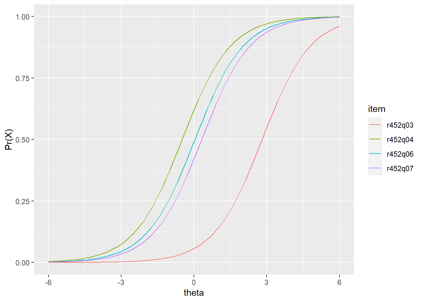
Figure 34.1: IRF for PISA09 reading items from “The play’s the thing” based on students in Great Britain.
Item pisagbr$r452q03s is estimated to be the most difficult for this set. The remaining three items in Figure 34.1 have locations or \(b\) parameters near theta 0. Notice that the IRF for these items, which come from the Rasch model, are all parallel, with the same slopes. They also have lower asymptotes of \(\Pr = 0\).
We can also use the results in irtgbr to examine SEM over theta. The SEM is obtained using the rtef() function from epmr. Figure 34.2 compares the SEM over theta for the full set of items (the black line), with SEM for subsets of 4 (blue) and 8 items (green). Fewer items at a given point in the theta scale also results in higher SEM at that theta. Thus, the number and location of items on the scale impact the resulting SEM.
# Plot SEM curve conditional on theta for full items
# Then add SEM for the subset of items 1:8 and 1:4
ggplot(rtef(irtgbr$ip), aes(theta, se)) + geom_line() +
  geom_line(aes(theta, se), data = rtef(irtgbr$ip[1:8, ]),
    col = "blue") +
  geom_line(aes(theta, se), data = rtef(irtgbr$ip[1:4, ]),
    col = "green")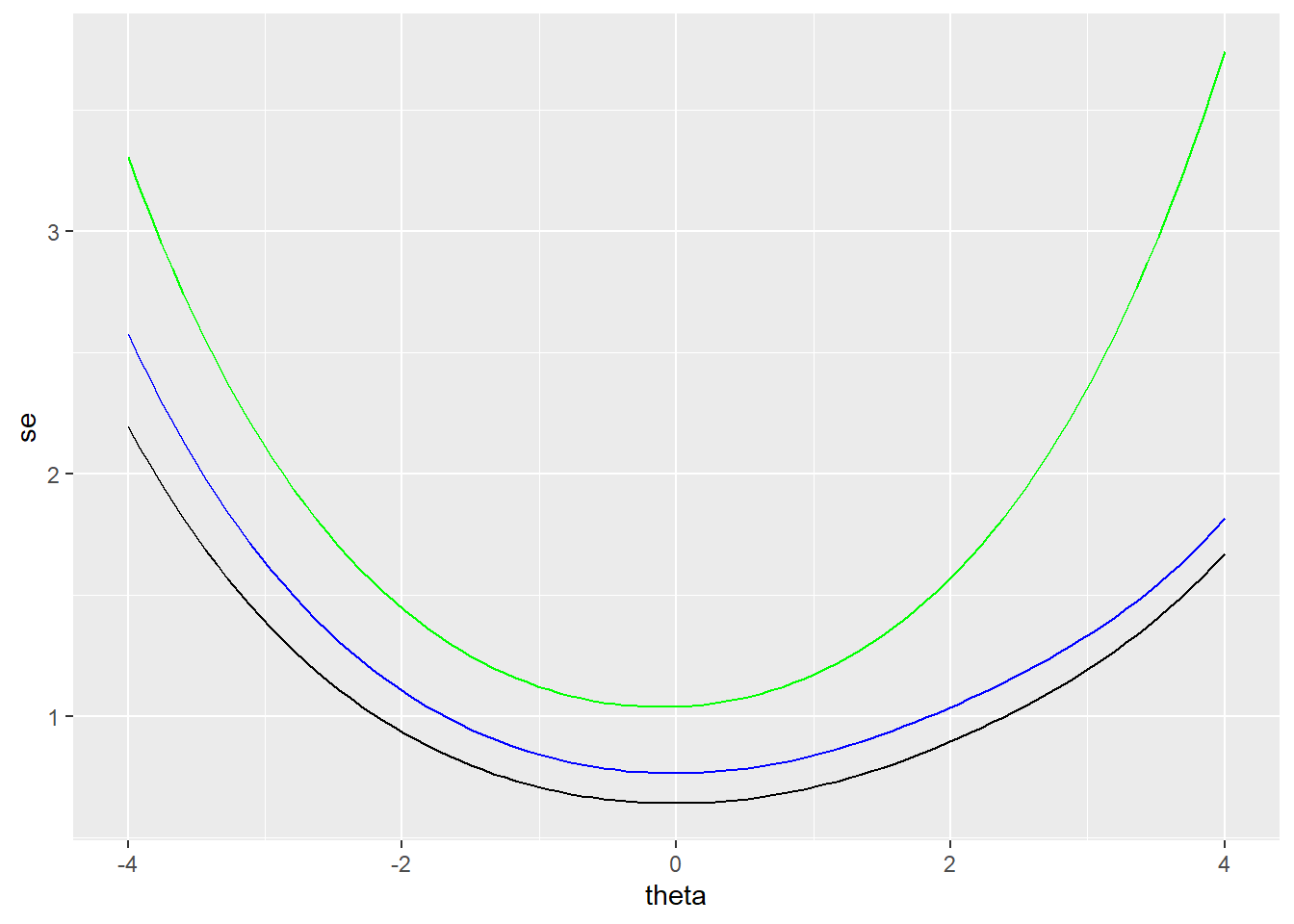
Figure 34.2: SEM for two subsets of PISA09 reading items based on students in Great Britain.
The rtef() function is used above with the default vector of theta seq(-4, 4, length = 100). However, SEM can be obtained for any theta based on the item parameters provided. Suppose we want to estimate the SEM for a high ability student who only takes low difficulty items. This constitutes a mismatch in item and construct, which produces a higher SEM. These SEM are interpreted like SEM from CTT, as the average variability we’d expect to see in a score due to measurement error. They can be used to build confidence intervals around theta for an individual.
# SEM for theta 3 based on the four easiest and the four
# most difficult items
rtef(irtgbr$ip[c(4, 6, 9, 11), ], theta = 3)
#>   theta  se
#> 1     3 2.9
rtef(irtgbr$ip[c(2, 7, 8, 10), ], theta = 3)
#>   theta se
#> 1     3  2
The reciprocal of the SEM function, via the TEF, is the test information function. This simply shows us where on the theta scale our test items are accumulating the most discrimination power, and, as a result, where measurement will be the most accurate. Higher information corresponds to higher accuracy and lower SEM. Figure 34.3 shows the test information for all the reading items, again based on students in Great Britain. Information is highest where SEM is lowest, at the center of the theta scale.
# Plot the test information function over theta
# Information is highest at the center of the theta scale
ggplot(rtif(irtgbr$ip), aes(theta, i)) + geom_line()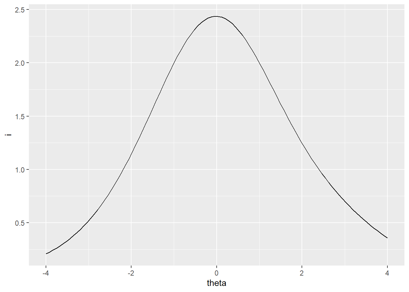
Figure 34.3: Test information for PISA09 reading items based on students in Great Britain.
Finally, just as the IRF can be used to predict probability of correct response on an item, given theta and the item parameters, the TRF can be used to predict total score given theta and parameters for each item in the test. The TRF lets us convert person theta back into the raw score metric for the test. Similar to the IRF, the TRF is asymptotic at 0 and the number of dichotomous items in the test, in this case, 11. Thus, no matter how high or how low theta, our predicted total score can’t exceed the bounds of the raw score scale. Figure 34.4 shows the test response function for the Great Britain results.
# Plot the test response function over theta
ggplot(rtrf(irtgbr$ip), aes(theta, p)) + geom_line()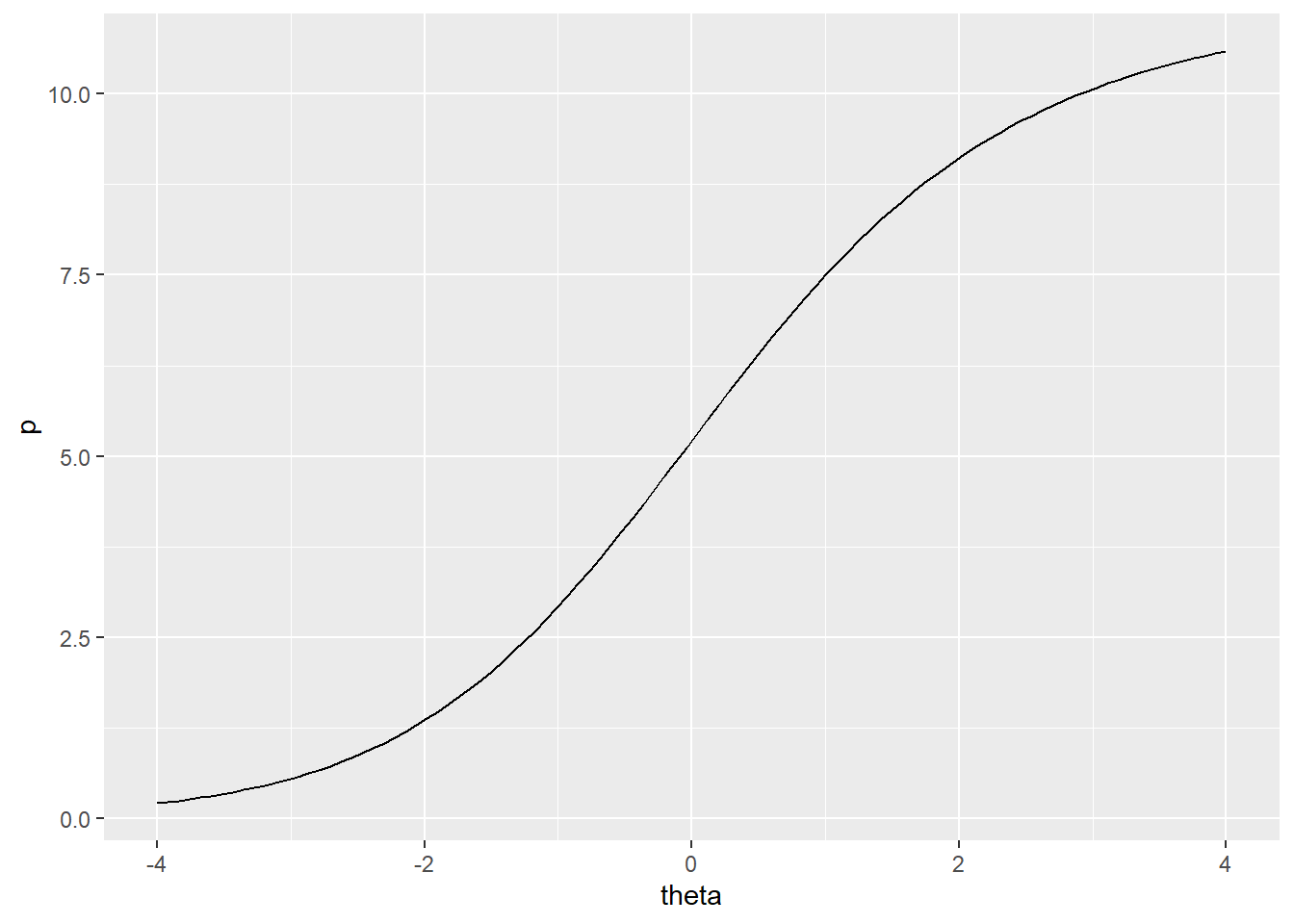
Figure 34.4: Test response function for PISA09 reading items based on students in Great Britain.