Extended: Plotting more complicated pedigrees with `ggPedigree()`
Source:vignettes/articles/v22_plots_morecomplexity.Rmd
v22_plots_morecomplexity.RmdIntroduction
This vignette demonstrates some of the more complex family trees you
can visualization with ggPedigree(). It extends the basic
examples found in the main package documentation.
We illustrate usage with a more complicated data set from ggpedigree:
asoiaf a fictional pedigree based on characters from the
A Song of Ice and Fire universe by George R. R. Martin. This
dataset includes complex relationships, such as half-siblings, multiple
marriages, and consanguineous relationships, making it an excellent
example for showcasing the capabilities of
ggPedigree().
Basic usage
# Install your package from GitHub

library(ggpedigree) # ggPedigree lives here
library(BGmisc) # helper utilities & example data
library(ggplot2) # ggplot2 for plotting
library(viridis) # viridis for color palettes
library(tidyverse) # for data wrangling
Load Packages and Data
We begin by loading the required libraries and examining the
structure of the built-in ASOIAF pedigree.
data(ASOIAF)The ASOIAF dataset includes character IDs, names, family identifiers, and parent identifiers for a subset of characters drawn from the A Song of Ice and Fire canon.
head(ASOIAF)
#>   id famID momID dadID          name sex
#> 1  1     1   566   564   Walder Frey   M
#> 2  2     1    NA    NA   Perra Royce   F
#> 3  3     1     2     1  Stevron Frey   M
#> 4  4     1     2     1    Emmon Frey   M
#> 5  5     1     2     1    Aenys Frey   M
#> 6  6     1    NA    NA Corenna Swann   F
#>                                                   url twinID zygosity
#> 1   https://awoiaf.westeros.org/index.php/Walder_Frey     NA     <NA>
#> 2   https://awoiaf.westeros.org/index.php/Perra_Royce     NA     <NA>
#> 3  https://awoiaf.westeros.org/index.php/Stevron_Frey     NA     <NA>
#> 4    https://awoiaf.westeros.org/index.php/Emmon_Frey     NA     <NA>
#> 5    https://awoiaf.westeros.org/index.php/Aenys_Frey     NA     <NA>
#> 6 https://awoiaf.westeros.org/index.php/Corenna_Swann     NA     <NA>
Data Cleaning
df_got <- checkSex(ASOIAF,
  code_male = "M",
  code_female = "F",
  repair = TRUE
)


# Find the IDs of Jon Snow and Daenerys Targaryen

jon_id <- df_got %>%
  filter(name == "Jon Snow") %>%
  pull(ID)

dany_id <- df_got %>%
  filter(name == "Daenerys Targaryen") %>%
  pull(ID)
Here we’ve added phantom IDs to the dataset, which are used to represent individuals who are not directly related to the family tree but are still part of the pedigree structure. This is useful for visualizing complex relationships, such as half-siblings or step-siblings.
df_repaired <- checkParentIDs(df_got,
  addphantoms = TRUE,
  repair = TRUE,
  parentswithoutrow = FALSE,
  repairsex = FALSE
) %>% mutate(
  famID_mulit = famID,
  famID = 1,
  affected = case_when(
    ID %in% c(jon_id, dany_id, "365") ~ 1,
    TRUE ~ 0
  )
)
#> REPAIR IN EARLY ALPHA
Visualize the Pedigree with kinship2
Here is the classic pedigree plot of the Targaryen family, with Jon
Snow and Daenerys Targaryen highlighted in black. The
kinship2_plotPedigree() function provides a quick way to
visualize the pedigree structure. It serves as a wrapper function from
{kinship2} and is useful for quickly checking the pedigree
structure.
library(kinship2)
kinship2_plotPedigree(df_repaired,
  affected = df_repaired$affected,
  verbose = FALSE
)
#> Did not plot the following people: 85 88 125 142 229 294 305 357 381 388 405 409 418 420 424 428 451 487 664
#> named list()
Visualize the Pedigree with ggPedigree()
Here is the same pedigree, but using ggPedigree() from
{ggpedigree}. This function provides a more flexible and customizable
way to visualize pedigrees, allowing for easy integration with other
ggplot2 functions.
df_repaired <- df_repaired %>% mutate(
  famID = famID_mulit
)

pltstatic <- ggPedigree(df_repaired,
  status_column = "affected",
  personID = "ID",
  config = list(
    return_static = TRUE,
    status_label_unaffected = 0,
    sex_color_include = FALSE,
    code_male = "M",
    point_size = 10,
    status_label_affected = 1,
    status_shape_affected = 4,
    ped_width = 14,
    tooltip_include = TRUE,
    label_nudge_y = .25,
    label_include = FALSE,
    label_method = "geom_text",
    #  segment_self_color = "purple",
    #   label_segment_color = "gray",
    reduce_variables = F,
    tooltip_columns = c("ID", "name")
  )
)

pltstatic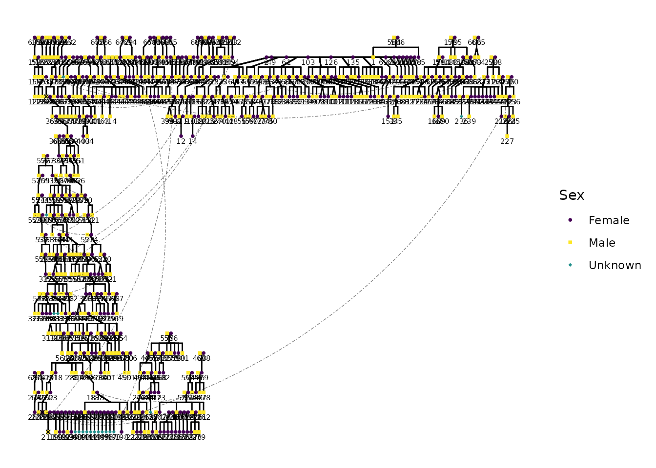
# pltstatic+ facet_wrap(~famID_mulit, drop=TRUE,scales = "free")
df_repaired_renamed <- df_repaired %>% rename(
  personID = ID
)
plt <- ggPedigreeInteractive(df_repaired_renamed,
  #  status_column = "affected",
  personID = "personID",
  # debug=TRUE,
  config = list(
    # status_label_unaffected = 0,
    sex_color_include = FALSE,
    focal_fill_personID = 353,
    focal_fill_include = TRUE,
    code_male = "M",
    point_size = 10,
    segment_linewidth = 0.25,
    status_include = FALSE,
    status_label_affected = 1,
    status_shape_affected = 4,
    ped_width = 14,
    #  segment_spouse_color = "red",
    #  segment_sibling_color = "blue",
    # segment_parent_color = "green",
    #  segment_offspring_color = "purple",
    # segment_self_color = NA,
    #  segment_mz_color = "orange",
    segment_self_angle = -75,
    segment_self_curvature = -0.15,
    focal_fill_force_zero = TRUE,
    focal_fill_mid_color = "orange",
    focal_fill_low_color = "#9F2A63FF",
    focal_fill_na_color = "black",
    focal_fill_use_log = TRUE,
    tooltip_include = TRUE,
    label_nudge_y = .25,
    label_include = TRUE,
    label_text_size = 1,
    label_method = "geom_text",
    segment_self_color = "black",
    tooltip_columns = c("personID", "name", "focal_fill")
  )
)

plt
htmlwidgets::saveWidget(plt, "ggpedigreeinteractive_aegon.html", selfcontained = TRUE)

plt <- ggPedigreeInteractive(df_repaired_renamed,
  #  status_column = "affected",
  personID = "personID",
  # debug=TRUE,
  config = list(
    # status_label_unaffected = 0,
    sex_color_include = FALSE,
    focal_fill_personID = 339,
    focal_fill_include = TRUE,
    code_male = "M",
    point_size = 10,
    segment_linewidth = 0.25,
    status_include = FALSE,
    status_label_affected = 1,
    status_shape_affected = 4,
    ped_width = 14,
    #  segment_spouse_color = "red",
    #  segment_sibling_color = "blue",
    # segment_parent_color = "green",
    #  segment_offspring_color = "purple",
    # segment_self_color = NA,
    #  segment_mz_color = "orange",
    segment_self_angle = -75,
    segment_self_curvature = -0.15,
    focal_fill_force_zero = TRUE,
    focal_fill_mid_color = "orange",
    focal_fill_low_color = "#9F2A63FF",
    focal_fill_na_color = "black",
    focal_fill_use_log = TRUE,
    tooltip_include = TRUE,
    label_nudge_y = .25,
    label_include = TRUE,
    label_text_size = 1,
    label_method = "geom_text",
    segment_self_color = "black",
    tooltip_columns = c("personID", "name", "focal_fill")
  )
)

plt
htmlwidgets::saveWidget(plt, "ggpedigreeinteractive_rh.html", selfcontained = TRUE)