Full Data Workflow

Introduction

This vignette provides a complete workflow for conducting discordant-kinship regression using the {discord} package. We encourage you to read the accompanying paper (Garrison et al., 2025) for a full explanation of the methods and their applications. Here, we demonstrate how to transform your data from its original structure into a format suitable for analysis, then walk through both standard OLS regression (for comparison) and discordant-kinship regression.

The tutorial covers three common starting data structures: wide format, long format, and pedigree data. We show how to prepare each for analysis using simulated data for reproducibility. You can adapt our analysis pipeline to your own data by substituting your variables and kinship links.

Data Structures and Preparation

Your data likely exists in one of three common formats (wide, long, or pedigree). Regardless of starting point, the goal is to create wide-format data where each row represents a kinship pair, with variables for each member of the pair distinguished by suffixes (e.g., _1 and _2). Understanding your data structure determines which transformation steps you’ll need.

Setup

First, load the necessary packages:

# For easy data manipulation
library(dplyr)
library(tidyr)

# For kinship linkages
library(NlsyLinks)
# For discordant-kinship regression
library(discord)
# To clean data frames
library(janitor)
library(broom)
# For pipe
library(magrittr)
# For pedigree data manipulation
library(BGmisc)
# For pedigree plotting
library(ggpedigree)
library(ggplot2)

Wide Format Data

Wide format is the most direct structure for our analysis. Each row represents one kinship pair, with variables appearing twice—once for each member of the pair—using suffixes to distinguish the two individuals. You’ll see columns like age_s1 and age_s2, where _s1 and _s2 identify which sibling’s data appears in each column.

Here’s an example with simulated sibling data:

df_wide <- data.frame(
  pid = 1:5,
  id_s1 = c(101, 201, 301, 401, 501),
  id_s2 = c(102, 202, 302, 402, 502),
  age_s1 = c(30, 27, 40, 36, 30),
  age_s2 = c(28, 25, 38, 35, 28),
  height_s1 = c(175, 160, 180, 170, 165),
  height_s2 = c(170, 162, 178, 172, 168),
  weight_s1 = c(70, 60, 80, 75, 65),
  weight_s2 = c(68, 62, 78, 74, 66)
)
df_wide %>%
  slice(1:5) %>%
  knitr::kable()

pid	id_s1	id_s2	age_s1	age_s2	height_s1	height_s2	weight_s1	weight_s2
1	101	102	30	28	175	170	70	68
2	201	202	27	25	160	162	60	62
3	301	302	40	38	180	178	80	78
4	401	402	36	35	170	172	75	74
5	501	502	30	28	165	168	65	66

In this example, pid is a unique identifier for each sibling pair. Specifically, each row is anchored by a pair identifier. Variables ending in _s1 refer to one sibling, while those ending in _s2 refer to the other. In this case, the dataset is already arranged so that the older sibling is _s1 and the younger is _s2, but this ordering will be adjusted later based on the outcome variable. If your data already has this structure, you can skip ahead to the “Ordering and Derived Variables” section.

Long Format Data Example

Long format structures data with one row per individual. In other words, each person appears in their own row, with a pair identifier column linking siblings together. This format is common in many datasets, particularly those downloaded from data repositories, but requires transformation for our analysis. For example, the NLSY datasets by default provide data in long format.

We can demonstrate long format by reshaping our wide data from above:

df_long <- df_wide %>%
  tidyr::pivot_longer(
    cols = -pid, # keep the dyad identifier intact
    names_to = c(".value", "sibling"), # split base names and the sibling marker
    names_sep = "_s" # original suffix delimiter in column names
  )

df_long %>%
  slice(1:10) %>%
  knitr::kable()

pid	sibling	id	age	height	weight
1	1	101	30	175	70
1	2	102	28	170	68
2	1	201	27	160	60
2	2	202	25	162	62
3	1	301	40	180	80
3	2	302	38	178	78
4	1	401	36	170	75
4	2	402	35	172	74
5	1	501	30	165	65
5	2	502	28	168	66

Notice how each individual now occupies their own row, with the sibling column indicating whether they were originally labeled 1 or 2. The pid column still identifies which individuals form a pair.

If your data does not already have a unique identifier for each kinship pair, you may need to construct your own based on the available information or download one from a kinship linkage resources. Ideally, you will also have information about the type of kinship (e.g., full siblings, half-siblings, cousins) and whether they were raised together or apart. (More on how to do this below for pedigree data.)

Converting Long to Wide

To convert long format data for discordant-kinship analysis, use pivot_wider() from the {tidyr} package:

df_long2wide <- df_long %>%
  tidyr::pivot_wider(
    names_from = sibling, # the column that indicates the sibling number
    values_from = c(id, age, height, weight), # variables to spread into paired columns
    names_sep = "_s" # ensures id_s1, id_s2,etc
  )

df_long2wide %>%
  slice(1:5) %>%
  knitr::kable()

pid	id_s1	id_s2	age_s1	age_s2	height_s1	height_s2	weight_s1	weight_s2
1	101	102	30	28	175	170	70	68
2	201	202	27	25	160	162	60	62
3	301	302	40	38	180	178	80	78
4	401	402	36	35	170	172	75	74
5	501	502	30	28	165	168	65	66

The reshaped data now reproduces our original wide format. Each analytic variable appears twice with _s1 and _s2 suffixes, and the pair identifier pid anchors each row.

Using existing kinship links

As mentioned before, if your long-format data lacks pair identifiers, you’ll need to create them using family IDs, household identifiers, or external kinship resources. This process can be straightforward if you have access to family or household identifiers, and are confident in the kinship relationships. However, it can be more complex if the relationships are not clearly defined or if there are multiple types of kinship (e.g., siblings, cousins, half-siblings) in your data.

For NLSY data specifically, the {NlsyLinks} package provides validated kinship links for the vast majority of dyads in the NLSY79 and NLSY97 cohorts. These links are provided in wide format, and can be used to left-join with the long-format data that the NLSY info website provides. See the {NlsyLinks} documentation for more details on how to access and use these datasets, or the reproducible source code for the analyses in the primary paper (Garrison et al., 2025).

library(NlsyLinks)
data(Links79PairExpanded)

Links79PairExpanded %>%
  arrange(ExtendedID) %>%
  filter(RelationshipPath == "Gen1Housemates" & RFull == 0.5) %>%
  slice_head(n = 5) %>%
  select(
    ExtendedID,
    SubjectTag_S1, SubjectTag_S2,
    RelationshipPath, RFull, IsMz,
    EverSharedHouse
  ) %>%
  knitr::kable()

ExtendedID	SubjectTag_S1	SubjectTag_S2	RelationshipPath	RFull	IsMz	EverSharedHouse
3	300	400	Gen1Housemates	0.5	No	TRUE
5	500	600	Gen1Housemates	0.5	No	TRUE
13	1300	1400	Gen1Housemates	0.5	No	TRUE
17	1700	1800	Gen1Housemates	0.5	No	TRUE
20	2000	2100	Gen1Housemates	0.5	No	TRUE

As you can see, this dataset includes an extended family identifier (ExtendedID), individual IDs for each sibling in the pair (R0000100 and R0000200), and their RelationshipPath (RelationshipPath = “Gen1Housemates” and genetic relatedness (RFull = 0.5). You can merge this dataset with your long-format data using the individual IDs.

At this stage the long‑origin data are indistinguishable from the original wide example. Each analytic variable now appears exactly twice—once for _s1 and once for _s2—and the dyad identifier pid continues to anchor the row. You can proceed directly to ordering and construction of *_mean and *_diff with discord_data().

Pedigree Data

Pedigree data is common in genetic and family studies, where detailed family trees are available. It is long format data that provides rich information about familial relationships, such as (mother ID, father ID, spouse ID). Our research team has developed specialized tools in the {BGmisc} package to extract kinship links and transform these pedigree structures into a wide format suitable for analysis. Below is an example of how such a dataset might look in both tabular and graphical forms:

data(potter)
ggpedigree(potter, config = list(
  label_method = "geom_text",
  label_nudge_y = .25,
  focal_fill_personID = 7,
  focal_fill_include = TRUE,
  focal_fill_force_zero = TRUE,
  focal_fill_na_value = "grey50",
  focal_fill_low_color = "darkred",
  focal_fill_high_color = "gold",
  focal_fill_mid_color = "orange",
  focal_fill_scale_midpoint = .65,
  focal_fill_component = "additive",
  focal_fill_method = "steps", #
  # focal_fill_method = "viridis_c",
  focal_fill_use_log = FALSE,
  focal_fill_n_breaks = 10,
  sex_color_include = TRUE,
  focal_fill_legend_title = "Genetic Relatives \nof Harry Potter"
)) +
  labs(title = "Potter Pedigree Plot") +
  theme(legend.position = "right")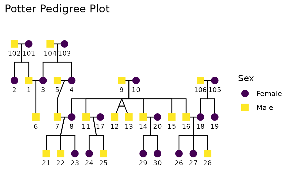

Pedigree plot of the Potter dataset

The pedigree tree above illustrates the family relationships among individuals in the Potter dataset. Each node represents an individual, and the lines connecting them indicate familial relationships such as parent-child and sibling connections.

data(potter)
df_ped <- potter %>%
  as.data.frame() %>%
  select(
    personID, sex, famID, momID, dadID, spouseID,
    twinID, zygosity
  ) %>%
  mutate(x_var = round(rnorm(nrow(.), mean = 0, sd = 1), digits = 2))

df_ped %>%
  slice(1:5) %>%
  knitr::kable(digits = 2)

personID	sex	famID	momID	dadID	spouseID	twinID	zygosity	x_var
1	1	1	101	102	3	NA	NA	-1.40
2	0	1	101	102	NA	NA	NA	0.26
3	0	1	103	104	1	NA	NA	-2.44
4	0	1	103	104	5	NA	NA	-0.01
5	1	1	NA	NA	4	NA	NA	0.62

As you can see, each individual is represented in a separate row, with columns for their unique identifier, mother’s identifier, father’s identifier, and other relevant variables.

{BGmisc} is available on CRAN and GitHub. It can create kinship links existing pedigree information.

To transform this data into a wide format suitable for discordant-kinship regression, we need to create kinship links based on the pedigree information. To extract the necessary kinship information, we need to compute two matrices: the additive genetic relatedness matrix and the shared environment matrix. Other matrices, such as mitochondrial, can also be computed if needed.

Using {BGmisc}, we compute:

The additive genetic relatedness matrix (add).
The shared environment matrix (cn), indicating whether kin were raised together (1) or apart (0).

add <- ped2add(df_ped)
cn <- ped2cn(df_ped)

The ped2add() function computes the additive genetic relatedness matrix, which quantifies the genetic similarity between individuals based on their pedigree information. The ped2cn() function computes the shared environment matrix, which indicates whether individuals were raised in the same environment (1) or different environments (0).

The resulting matrices are symmetric, with diagonal elements representing self-relatedness (1.0). The off-diagonal elements represent the relatedness between pairs of individuals, with values ranging from 0 (no relatedness) to 0.5 (full siblings) to 1 (themselves).

We convert the component matrices into a wide-form dataframe of kin pairs using com2links(). Self-pairs and duplicate entries are removed.

df_links <- com2links(
  writetodisk = FALSE,
  ad_ped_matrix = add,
  cn_ped_matrix = cn,
  drop_upper_triangular = TRUE
) %>%
  filter(ID1 != ID2)

df_links %>%
  slice(1:5) %>%
  knitr::kable(digits = 3)

ID1	ID2	addRel	cnuRel
1	2	0.50	1
3	4	0.50	1
1	6	0.50	0
2	6	0.25	0
3	6	0.50	0

As you can see, the df_links data frame contains pairs of individuals (ID1 and ID2) along with their additive genetic relatedness (addRel) and shared environment status (cnuRel). These data are in wide format, with each row representing a unique pair of individuals.

Further, we can tally the number of pairs by relatedness and shared environment to understand the composition of the dataset.

df_links %>%
  group_by(addRel, cnuRel) %>%
  tally() %>%
  knitr::kable()

addRel	cnuRel	n
0.0625	0	3
0.1250	0	47
0.2500	0	104
0.5000	0	50
0.5000	1	32

This table shows the number of kinship pairs for each combination of genetic relatedness and shared environment status. Although the discord regression model can be used with any kin group, it is most interpretable when there is a single kinship group.

For demonstration, we’ll focus on first cousins raised in separate homes from our pedigree data. This subset allows us to illustrate the process clearly.

set.seed(2024)
df_cousin <- df_links %>%
  filter(addRel == .125) %>% # only cousins %>%
  filter(cnuRel == 0) # only kin raised in separate homes

df_synthetic <- discord::kinsim(
  mu_all = c(1, 1),
  cov_a = .5,
  cov_c = .1,
  cov_e = .3,
  c_vector = rep(df_cousin$cnuRel, 3),
  r_vector = rep(df_cousin$addRel, 3)
) %>%
  select(
    pid = id,
    r,
    weight_s1 = y1_1,
    weight_s2 = y1_2,
    height_s1 = y2_1,
    height_s2 = y2_2
  ) %>%
  mutate(
    age_s1 = round(rnorm(nrow(.), mean = 30, sd = 5), digits = 0),
    age_s2 = age_s1 - sample(1:5, nrow(.), replace = TRUE)
  )

df_synthetic %>%
  slice(1:5) %>%
  knitr::kable(digits = 2)

pid	r	weight_s1	weight_s2	height_s1	height_s2	age_s1	age_s2
1	0.12	2.09	-1.30	4.54	-0.66	31	30
2	0.12	1.21	0.40	1.20	0.26	32	28
3	0.12	1.03	2.53	2.76	0.58	29	27
4	0.12	1.46	4.92	0.93	-0.67	30	29
5	0.12	2.69	2.78	0.95	-0.54	23	18

Ordering and Derived Variables

Now that we have our data in wide format, we can proceed to order the pairs and create the derived variables needed for discordant-kinship regression. The key steps are:

Ordering the pairs: We need to ensure that within each pair, the individual with the higher outcome value is consistently labeled as _1 and the other as _2. This ordering is to ensure that we can extract meaningful difference scores.
Creating derived variables: We will create *_mean and *_diff* variables for both the outcome and predictor variables. The *_mean variable represents the average of the two individuals’ values, while the *_diff variable represents the difference between the two individuals’ values (i.e., _1 - _2).

These steps can be accomplished using the discord_data() function from the {discord} package. This function takes care of ordering the pairs and creating the derived variables, ensuring that the data is ready for analysis. When using discord_data(), you will need to specify the outcome variable, predictor variables, and the identifiers for the two members of each pair.

Below we default to the long path for reproducibility. Replace with your chosen source as needed.

# CHOOSE ONE based on your path
# source_wide <- df_wide
# source_wide <- df_long2wide
source_wide <- df_synthetic # if you followed the pedigree path

Now call discord_data() specifying the outcome and predictor present for both siblings. Here we use Y as the outcome and X as the predictor, with your _S1 / _S2 suffix convention.

df_discord_weight <- discord::discord_data(
  data = source_wide,
  outcome = "weight",
  predictors = c("height", "age"),
  demographics = "none",
  pair_identifiers = c("_s1", "_s2"),
  id = "pid" # or "famID" if you followed the pedigree path
)

df_discord_weight %>%
  slice(1:5) %>%
  knitr::kable(digits = 2, caption = "Transformed data ready for discordant-kinship regression")

Transformed data ready for discordant-kinship regression
id	weight_1	weight_2	weight_diff	weight_mean	height_1	height_2	height_diff	height_mean	age_1	age_2	age_diff	age_mean
1	2.09	-1.30	3.39	0.39	4.54	-0.66	5.20	1.94	31	30	1	30.5
2	1.21	0.40	0.81	0.80	1.20	0.26	0.94	0.73	32	28	4	30.0
3	2.53	1.03	1.51	1.78	0.58	2.76	-2.18	1.67	27	29	-2	28.0
4	4.92	1.46	3.46	3.19	-0.67	0.93	-1.60	0.13	29	30	-1	29.5
5	2.78	2.69	0.09	2.74	-0.54	0.95	-1.49	0.21	18	23	-5	20.5

Understanding the Transformation

Let’s examine what discord_data() did to our variables:

df_discord_weight %>%
  select(
    id,
    weight_1, weight_2, weight_mean, weight_diff,
    height_1, height_2, height_mean, height_diff
  ) %>%
  slice(1:5) %>%
  knitr::kable(digits = 2)

id	weight_1	weight_2	weight_mean	weight_diff	height_1	height_2	height_mean	height_diff
1	2.09	-1.30	0.39	3.39	4.54	-0.66	1.94	5.20
2	1.21	0.40	0.80	0.81	1.20	0.26	0.73	0.94
3	2.53	1.03	1.78	1.51	0.58	2.76	1.67	-2.18
4	4.92	1.46	3.19	3.46	-0.67	0.93	0.13	-1.60
5	2.78	2.69	2.74	0.09	-0.54	0.95	0.21	-1.49

Notice several important patterns in this output. First, weight_1 is always greater than or equal to weight_2 because discord_data() ordered siblings by the outcome variable. The sibling with higher weight becomes _1 and the sibling with lower weight becomes _2. This ordering ensures that weight_diff (calculated as weight_1 - weight_2) is always non-negative.

Second, the mean scores represent each pair’s average. For example, weight_mean equals the average of weight_1 and weight_2. These means capture between-family variation - how pairs differ from each other in average weight.

Third, the predictor differences can be positive or negative. Even though weight differences are always positive (by construction), height differences vary. The taller sibling might be the heavier one, or the shorter sibling might be heavier. This variation is what we’ll test in our regression.

This structure lets us ask a key question: within sibling pairs, does the sibling with more of the predictor also have more of the outcome? If the taller sibling is systematically heavier even after controlling for family background, that suggests height may causally influence weight. If not, the association likely reflects familial confounding.

Analyzing the Data

With our data prepared, we can now perform both standard OLS regression and discordant-kinship regression to compare results.

Standard OLS Regression

First, let’s run a standard OLS regression using the original wide-format data. This will serve as a baseline for comparison with the family-based analyses.

For our baseline analysis, we select one sibling from each pair. In the original dataset, s1 was defined as the older sibling, so we can simply choose the sibling labeled _s1. But, another way to select the oldest sibling is to use the discord_data() function with the outcome argument set to the age variable. This will ensure that _1 is always the oldest sibling within the pair. In the case of ties, one sibling is randomly assigned as _1.

df_for_ols <- df_synthetic %>%
  dplyr::select(
    id = pid,
    weight = weight_s1,
    height = height_s1,
    age = age_s1
  )


df_discord_age <- discord::discord_data(
  data = source_wide,
  outcome = "age",
  predictors = c("height", "weight"),
  demographics = "none",
  pair_identifiers = c("_s1", "_s2"),
  id = "pid" # or "famID" if you followed the pedigree path
)

df_discord_age %>%
  select(
    id, age_1, age_2,
    age_mean, age_diff, weight_1, height_1
  ) %>%
  slice(1:5) %>%
  knitr::kable(caption = "One sibling per pair for OLS regression, selecting by age", digits = 2)

One sibling per pair for OLS regression, selecting by age
id	age_1	age_2	age_mean	age_diff	weight_1	height_1
1	31	30	30.5	1	2.09	4.54
2	32	28	30.0	4	1.21	1.20
3	29	27	28.0	2	1.03	2.76
4	30	29	29.5	1	1.46	0.93
5	23	18	20.5	5	2.69	0.95


df_for_ols %>%
  select(id, age, weight, height) %>%
  slice(1:5) %>%
  knitr::kable(caption = "One sibling per pair for OLS regression using original wide data", digits = 2)

One sibling per pair for OLS regression using original wide data
id	age	weight	height
1	31	2.09	4.54
2	32	1.21	1.20
3	29	1.03	2.76
4	30	1.46	0.93
5	23	2.69	0.95

As you can see, df_for_ols and df_discord_age both resulted in the same individuals being selected for analysis. The df_discord_age dataset was created by ordering siblings based on age, ensuring that _1 is always the older sibling. The df_for_ols dataset directly selects the older sibling from the original wide data.

By selecting one sibling per pair, we’re analyzing the same number of observations as we have kinship pairs. This represents the standard individual-level approach used in most research:

$$ Y = \\beta_0 + \\beta_1 X1 + \\beta_2 X2 + \\epsilon $$

ols_model <- lm(weight ~ height + age, data = df_for_ols)

stargazer::stargazer(ols_model,
  type = "html",
  digits = 3, single.row = TRUE, title = "Standard OLS Regression Results"
)

**Standard OLS Regression Results**

	Dependent variable:

	weight

height	0.287^*** (0.078)
age	-0.073^** (0.029)
Constant	2.788^*** (0.871)

Observations	141
R²	0.125
Adjusted R²	0.112
Residual Std. Error	1.573 (df = 138)
F Statistic	9.857^*** (df = 2; 138)

Note:	p<0.1; p<0.05; p<0.01

This standard regression shows associations between our variables while controlling only for measured covariates.

Discordant Between-Family Regression

Next, we run a between-family regression using the discordant data. This model regresses the outcome mean on predictor means, capturing between-family variation:

$$ Y_{mean} = \\beta_0 + \\beta_1 X1_{mean} + \\beta_2 X2_{mean} + \\epsilon $$

between_model <- lm(
  weight_mean ~ height_mean + age_mean,
  data = df_discord_weight
)

stargazer::stargazer(between_model,
  type = "html",
  digits = 3, single.row = TRUE, title = "Between-Family Regression Results"
)

**Between-Family Regression Results**

	Dependent variable:

	weight_mean

height_mean	0.199^** (0.077)
age_mean	-0.044^* (0.023)
Constant	2.064^*** (0.666)

Observations	141
R²	0.067
Adjusted R²	0.054
Residual Std. Error	1.284 (df = 138)
F Statistic	4.970^*** (df = 2; 138)

Note:	p<0.1; p<0.05; p<0.01

This between-family regression captures how differences in average height and age across families relate to average weight. However, it does not account for within-family differences, which is where discordant-kinship regression comes in.

It is important to note that the between-family regression results are not directly comparable to the standard OLS regression results. The between-family model uses mean scores, which represent family-level averages, while the OLS model uses individual-level data. Therefore, the coefficients from these two models may differ in magnitude and interpretation. But, they both provide useful information about the relationships among the variables.

Discordant-Kinship Regression

Now we return to our prepared data to run discordant-kinship regression. We can specify the models manually or use the discord_regression() convenience function. Both approaches produce identical results.

The discordant model regresses the outcome difference on outcome mean, predictor means, and predictor differences:

$$ Y_{diff} = \\beta_0 + \\beta_1 Y_{mean} + \\beta_2 X1_{mean} + \\beta_3 X1_{diff} + \\beta_4 X2_{mean} + \\beta_5 X2_{diff} + \\epsilon $$

discord_model_manual <- lm(
  weight_diff ~ weight_mean + height_mean + height_diff + age_mean + age_diff,
  data = df_discord_weight
)

tidy(discord_model_manual, conf.int = TRUE) %>%
  knitr::kable(digits = 3, caption = "Discordant Regression (Manual)")

Discordant Regression (Manual)
term	estimate	std.error	statistic	p.value	conf.low	conf.high
(Intercept)	0.500	0.528	0.948	0.345	-0.544	1.544
weight_mean	-0.043	0.065	-0.660	0.511	-0.171	0.086
height_mean	0.041	0.060	0.680	0.498	-0.078	0.159
height_diff	0.141	0.043	3.254	0.001	0.055	0.226
age_mean	0.031	0.018	1.742	0.084	-0.004	0.066
age_diff	-0.026	0.024	-1.092	0.277	-0.074	0.021

stargazer::stargazer(between_model, discord_model_manual,
  type = "html",
  digits = 3, single.row = TRUE, title = "Between-Family and Discordant Regression Results"
)

**Between-Family and Discordant Regression Results**

	Dependent variable:

	weight_mean	weight_diff
	(1)	(2)

weight_mean		-0.043 (0.065)
height_mean	0.199^** (0.077)	0.041 (0.060)
height_diff		0.141^*** (0.043)
age_mean	-0.044^* (0.023)	0.031^* (0.018)
age_diff		-0.026 (0.024)
Constant	2.064^*** (0.666)	0.500 (0.528)

Observations	141	141
R²	0.067	0.102
Adjusted R²	0.054	0.069
Residual Std. Error	1.284 (df = 138)	0.978 (df = 135)
F Statistic	4.970^*** (df = 2; 138)	3.060^** (df = 5; 135)

Note:	p<0.1; p<0.05; p<0.01

Note that we are using the df_discord_weight dataset created earlier with discord_data(). This dataset is ordered such that within a pair, the sibling with the higher weight is always _1. This ordering ensures that weight_diff is always non-negative, which is a key feature of discordant-kinship regression.

Using the Helper Function

Alternatively, we can use the discord_regression() function, which simplifies the process:

By default, discord_regression() orders siblings by the outcome variable, creates the necessary derived variables, and fits the discordant regression model in one step. This function also allows for easy inclusion of demographic covariates if needed. See the function documentation for more details on these options, as well as a vignette focused on demographic controls.

discord_model <- discord_regression(
  data = source_wide,
  outcome = "weight",
  predictors = c("height", "age"),
  demographics = "none",
  sex = NULL,
  race = NULL,
  pair_identifiers = c("_s1", "_s2"),
  id = "pid"
)

tidy(discord_model, conf.int = TRUE) %>%
  knitr::kable(digits = 3, caption = "Discordant Regression Results")

Discordant Regression Results
term	estimate	std.error	statistic	p.value	conf.low	conf.high
(Intercept)	0.500	0.528	0.948	0.345	-0.544	1.544
weight_mean	-0.043	0.065	-0.660	0.511	-0.171	0.086
height_diff	0.141	0.043	3.254	0.001	0.055	0.226
age_diff	-0.026	0.024	-1.092	0.277	-0.074	0.021
height_mean	0.041	0.060	0.680	0.498	-0.078	0.159
age_mean	0.031	0.018	1.742	0.084	-0.004	0.066


glance(discord_model) %>%
  select(r.squared, adj.r.squared, sigma, p.value, nobs) %>%
  knitr::kable(digits = 3)

r.squared	adj.r.squared	sigma	p.value	nobs
0.102	0.069	0.978	0.012	141

stargazer::stargazer(discord_model,
  discord_model_manual,
  type = "html",
  digits = 3, single.row = TRUE, title = "Discordant Regression Results Comparison"
)

% Error: Unrecognized object type.

Session Info

sessioninfo::session_info()
#> ─ Session info ───────────────────────────────────────────────────────────────
#>  setting  value
#>  version  R version 4.5.1 (2025-06-13)
#>  os       Ubuntu 24.04.3 LTS
#>  system   x86_64, linux-gnu
#>  ui       X11
#>  language en
#>  collate  C.UTF-8
#>  ctype    C.UTF-8
#>  tz       UTC
#>  date     2025-10-06
#>  pandoc   3.1.11 @ /opt/hostedtoolcache/pandoc/3.1.11/x64/ (via rmarkdown)
#>  quarto   NA
#> 
#> ─ Packages ───────────────────────────────────────────────────────────────────
#>  package      * version date (UTC) lib source
#>  backports      1.5.0   2024-05-23 [1] RSPM
#>  BGmisc       * 1.5.0   2025-07-19 [1] RSPM
#>  broom        * 1.0.10  2025-09-13 [1] RSPM
#>  bslib          0.9.0   2025-01-30 [1] RSPM
#>  cachem         1.1.0   2024-05-16 [1] RSPM
#>  cli            3.6.5   2025-04-23 [1] RSPM
#>  data.table     1.17.8  2025-07-10 [1] RSPM
#>  desc           1.4.3   2023-12-10 [1] RSPM
#>  digest         0.6.37  2024-08-19 [1] RSPM
#>  discord      * 1.3     2025-10-06 [1] local
#>  dplyr        * 1.1.4   2023-11-17 [1] RSPM
#>  evaluate       1.0.5   2025-08-27 [1] RSPM
#>  farver         2.1.2   2024-05-13 [1] RSPM
#>  fastmap        1.2.0   2024-05-15 [1] RSPM
#>  fs             1.6.6   2025-04-12 [1] RSPM
#>  generics       0.1.4   2025-05-09 [1] RSPM
#>  ggpedigree   * 0.9.0   2025-09-12 [1] RSPM
#>  ggplot2      * 4.0.0   2025-09-11 [1] RSPM
#>  glue           1.8.0   2024-09-30 [1] RSPM
#>  gtable         0.3.6   2024-10-25 [1] RSPM
#>  htmltools      0.5.8.1 2024-04-04 [1] RSPM
#>  htmlwidgets    1.6.4   2023-12-06 [1] RSPM
#>  janitor      * 2.2.1   2024-12-22 [1] RSPM
#>  jquerylib      0.1.4   2021-04-26 [1] RSPM
#>  jsonlite       2.0.0   2025-03-27 [1] RSPM
#>  kinship2       1.9.6.2 2025-09-04 [1] RSPM
#>  knitr          1.50    2025-03-16 [1] RSPM
#>  labeling       0.4.3   2023-08-29 [1] RSPM
#>  lattice        0.22-7  2025-04-02 [3] CRAN (R 4.5.1)
#>  lifecycle      1.0.4   2023-11-07 [1] RSPM
#>  lubridate      1.9.4   2024-12-08 [1] RSPM
#>  magrittr     * 2.0.4   2025-09-12 [1] RSPM
#>  Matrix         1.7-3   2025-03-11 [3] CRAN (R 4.5.1)
#>  NlsyLinks    * 2.2.3   2025-08-31 [1] RSPM
#>  pillar         1.11.1  2025-09-17 [1] RSPM
#>  pkgconfig      2.0.3   2019-09-22 [1] RSPM
#>  pkgdown        2.1.3   2025-05-25 [1] any (@2.1.3)
#>  purrr          1.1.0   2025-07-10 [1] RSPM
#>  quadprog       1.5-8   2019-11-20 [1] RSPM
#>  R6             2.6.1   2025-02-15 [1] RSPM
#>  ragg           1.5.0   2025-09-02 [1] RSPM
#>  RColorBrewer   1.1-3   2022-04-03 [1] RSPM
#>  rlang          1.1.6   2025-04-11 [1] RSPM
#>  rmarkdown      2.30    2025-09-28 [1] RSPM
#>  S7             0.2.0   2024-11-07 [1] RSPM
#>  sass           0.4.10  2025-04-11 [1] RSPM
#>  scales         1.4.0   2025-04-24 [1] RSPM
#>  sessioninfo    1.2.3   2025-02-05 [1] any (@1.2.3)
#>  snakecase      0.11.1  2023-08-27 [1] RSPM
#>  stargazer      5.2.3   2022-03-04 [1] RSPM
#>  stringi        1.8.7   2025-03-27 [1] RSPM
#>  stringr        1.5.2   2025-09-08 [1] RSPM
#>  systemfonts    1.3.1   2025-10-01 [1] RSPM
#>  textshaping    1.0.3   2025-09-02 [1] RSPM
#>  tibble         3.3.0   2025-06-08 [1] RSPM
#>  tidyr        * 1.3.1   2024-01-24 [1] RSPM
#>  tidyselect     1.2.1   2024-03-11 [1] RSPM
#>  timechange     0.3.0   2024-01-18 [1] RSPM
#>  vctrs          0.6.5   2023-12-01 [1] RSPM
#>  withr          3.0.2   2024-10-28 [1] RSPM
#>  xfun           0.53    2025-08-19 [1] RSPM
#>  yaml           2.3.10  2024-07-26 [1] RSPM
#> 
#>  [1] /home/runner/work/_temp/Library
#>  [2] /opt/R/4.5.1/lib/R/site-library
#>  [3] /opt/R/4.5.1/lib/R/library
#>  * ── Packages attached to the search path.
#> 
#> ──────────────────────────────────────────────────────────────────────────────

pid	id_s1	id_s2	age_s1	age_s2	height_s1	height_s2	weight_s1	weight_s2
1	101	102	30	28	175	170	70	68
2	201	202	27	25	160	162	60	62
3	301	302	40	38	180	178	80	78
4	401	402	36	35	170	172	75	74
5	501	502	30	28	165	168	65	66

pid	sibling	id	age	height	weight
1	1	101	30	175	70
1	2	102	28	170	68
2	1	201	27	160	60
2	2	202	25	162	62
3	1	301	40	180	80
3	2	302	38	178	78
4	1	401	36	170	75
4	2	402	35	172	74
5	1	501	30	165	65
5	2	502	28	168	66

pid	id_s1	id_s2	age_s1	age_s2	height_s1	height_s2	weight_s1	weight_s2
1	101	102	30	28	175	170	70	68
2	201	202	27	25	160	162	60	62
3	301	302	40	38	180	178	80	78
4	401	402	36	35	170	172	75	74
5	501	502	30	28	165	168	65	66

pid	id_s1	id_s2	age_s1	age_s2	height_s1	height_s2	weight_s1	weight_s2
1	101	102	30	28	175	170	70	68
2	201	202	27	25	160	162	60	62
3	301	302	40	38	180	178	80	78
4	401	402	36	35	170	172	75	74
5	501	502	30	28	165	168	65	66

pid	sibling	id	age	height	weight
1	1	101	30	175	70
1	2	102	28	170	68
2	1	201	27	160	60
2	2	202	25	162	62
3	1	301	40	180	80
3	2	302	38	178	78
4	1	401	36	170	75
4	2	402	35	172	74
5	1	501	30	165	65
5	2	502	28	168	66

pid	id_s1	id_s2	age_s1	age_s2	height_s1	height_s2	weight_s1	weight_s2
1	101	102	30	28	175	170	70	68
2	201	202	27	25	160	162	60	62
3	301	302	40	38	180	178	80	78
4	401	402	36	35	170	172	75	74
5	501	502	30	28	165	168	65	66

S. Mason Garrison