Power Analysis for Discordant Sibling Designs

Introduction

This vignette demonstrates how to conduct simulation-based power analysis for discordant sibling designs. These designs estimate causal effects by comparing differences between genetically related individuals, controlling for shared background.

We simulate multivariate phenotypes using the kinsim() function, fit regression models of interest, and calculate empirical power across multiple design conditions.

Function Overview: kinsim()

The kinsim() function is designed to simulate data for kinship studies. It generates paired multivariate data informed by biometric models (ACE), supporting variable relatedness levels and covariance structures.

Key Arguments

Argument	Description
`r_all`	Vector of genetic relatedness values (e.g., `1`, `0.5`, `0.25`, `0`)
`c_all`	Vector of shared environmental correlations (e.g., `1`, `1`,`0`, `0`)
`npergroup_all`	Sample sizes for each level of relatedness
`ace_list`	Matrix of ACE parameters per variable (rows = traits; columns = a, c, e)
`cov_a`, `cov_c`, `cov_e`	Cross-variable covariance for A, C, and E components
`mu_list`	Mean values for each phenotype
`r_vector`	Optional: pairwise relatedness at the observation level

Output

A data.frame with:

Latent variables: A, C, E for each phenotype and sibling
Phenotypic outcomes: y1 and y2 for both phenotypes
Metadata: relatedness level (r) and pair id

Example Usage

Step 1: Define Simulation Grid

We define a grid of simulation conditions, varying genetic relatedness, ACE variance components, and genetic correlations.

# Libraries
library(NlsyLinks)
library(discord)
library(utils)
library(tidyverse)
library(ggplot2)
# Set random seed for reproducibility
set.seed(1492)

# Disable scientific notation for clarity
options(scipen = 999)


conditions <- expand.grid(
  id = 1,
  total_pairs = c(100, 250, 500, 750, 1000),
  relatedness = c(1, .5),
  raised_together = c(1), # 1 if raised together, 0 if apart
  cov_a = c(0, 0.25),
  cov_c = c(0, 0.25),
  cov_e = c(0, 0.25),
  ace_a = c(1),
  ace_c = c(1),
  ace_e = c(1)
)
conditions$id <- 1:nrow(conditions)

Here, we vary the total number of sibling pairs, genetic relatedness (MZ vs. DZ), and the presence/absence of covariates influencing the phenotypes through A, C, and E pathways. The ACE variance components are held constant at 1 for simplicity. This results in a total of 80 unique conditions to evaluate.

Step 2: Run Simulations

For each condition, we simulate 100 replications of fitting discordant sibling models. We have kept the number of trials low for demonstration purposes, but you can and should increase n_trials for more robust power estimates, the normal recommendation is at least 1000 trials.

Please note that the simulations may take some time to run, especially with larger sample sizes and more trials. Also note that the FAST option can be set to TRUE for quicker, less detailed analyses, or FALSE for more thorough analyses. The FAST option drops pairs that are tied on the outcome, because it filters only to pairs where the outcome difference is greater than zero.

# Set number of trials (increase for more robust estimates)
n_trials <- 100


set.seed(1492) # Set seed for reproducibility
FAST <- FALSE # Set to FALSE for slower, more detailed analysis
results_list <- list()
name.results <- c("coef_xdiff", "p_xdiff", "r.squared")

for (cond in seq_along(conditions$id)) {
  current <- conditions[cond, ]
  temp_results <- matrix(NA, nrow = n_trials, ncol = length(name.results))
  colnames(temp_results) <- name.results

  for (i in 1:n_trials) {
    trial <- kinsim(
      r_all = current$relatedness,
      c_all = current$raised_together,
      npg_all = current$total_pairs,
      mu_list = c(1, 1),
      ace_all = c(current$ace_a, current$ace_c, current$ace_e),
      cov_a = current$cov_a,
      cov_c = current$cov_c,
      cov_e = current$cov_e,
      variables = 2
    )

    extract <- data.frame(
      id = trial$id, r = trial$r,
      y_s1 = trial$y1_1, y_s2 = trial$y1_2,
      x_s1 = trial$y2_1, x_s2 = trial$y2_2
    )
# 
    if (FAST == TRUE) {
      # faster
      # double enter the data and subset to ydiff > 0
      extract2 <- rbind(
        transform(extract,
          y_s1 = y_s2, y_s2 = y_s1,
          x_s1 = x_s2, x_s2 = x_s1
        ),
        extract
      )
      extract2$y_diff <- extract2$y_s1 - extract2$y_s2
      extract2$x_diff <- extract2$x_s1 - extract2$x_s2
      extract2$x_bar <- (extract2$x_s1 + extract2$x_s2) / 2
      extract2$y_bar <- (extract2$y_s1 + extract2$y_s2) / 2

      # select pair with ydiff > 0
      extract3 <- extract2[extract2$y_diff > 0, ]

      fit <- tryCatch(
        lm(y_diff ~ x_bar + y_bar + x_diff, data = extract3),
        error = function(e) {
          return(NULL)
        }
      )
    }
    # slower
    if (FAST == FALSE) {
      fit <- tryCatch(
        discord_regression(
          data = extract, outcome = "y", predictors = "x",
          id = "id",
          sex = NULL,
          race = NULL,
          fast = TRUE
        ),
        error = function(e) {
          return(NULL)
        }
      )
    }
    if (!is.null(fit)) {
      sm <- summary(fit)
      temp_results[i, "coef_xdiff"] <- coef(sm)["x_diff", "Estimate"]
      temp_results[i, "p_xdiff"] <- coef(sm)["x_diff", "Pr(>|t|)"]
      temp_results[i, "r.squared"] <- sm$r.squared
    }
  }

  results_list[[cond]] <- as.data.frame(temp_results)
}

Step 3: Summarize Power

Our final step is to summarize the power across all conditions. We calculate the proportion of trials where the p-value for the difference in means (p_xdiff) is less than 0.05, and we also report the median R-squared value from the regression models. Note that we’ve limited the number of trials to 100 for demonstration purposes, but you can (and should) increase this for more robust estimates.

power_summary <- lapply(results_list, function(res) {
  data.frame(
    effect_detected = sum(res$p_xdiff < 0.05, na.rm = TRUE),
    effect_notdetected = sum(res$p_xdiff >= 0.05, na.rm = TRUE),
    total = sum(!is.na(res$p_xdiff)),
    power_xdiff = mean(res$p_xdiff < 0.05, na.rm = TRUE),
    median_r2   = median(res$r.squared, na.rm = TRUE)
  )
})

final_results <- cbind(conditions, do.call(rbind, power_summary))

Step 4: Visualize Power

We can visualize the power estimates across different conditions. The plots below show the power estimates for each condition, including the total number of pairs, relatedness level, covariate settings, and the median R-squared value from the regression models. As expected, power increases with the number of pairs and is influenced by the relatedness level and covariate settings. In the plots below, we visualize the power estimates across different conditions, focusing on the impact of covariates and relatedness levels.

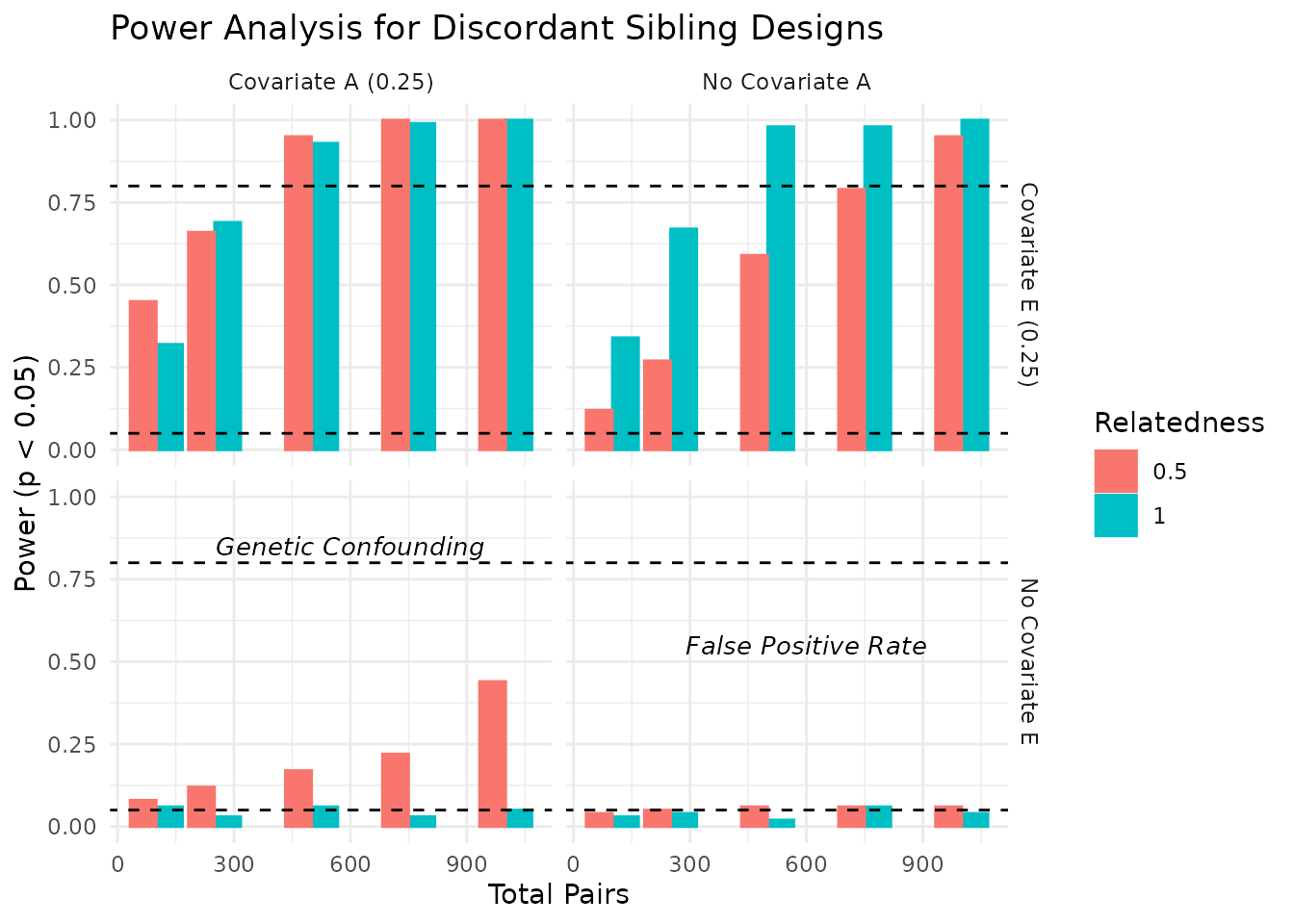
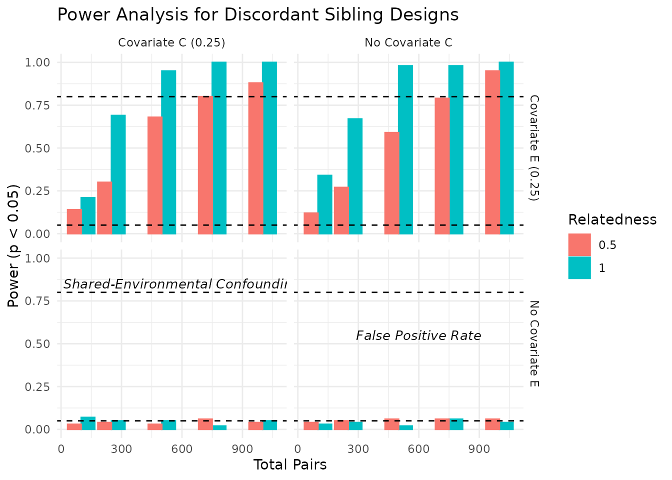
In the plots above, we see how power varies with the number of sibling pairs, relatedness levels, and the presence of covariates. The dashed lines indicate common benchmarks for power (0.80) and false positive rate (0.05). As expected, power increases with the number of pairs and is influenced by the relatedness level and covariate settings.

Power Table

The table below summarizes the power estimates across different conditions. The power_xdiff column indicates the proportion of trials where the p-value for the difference in means (p_xdiff) is less than 0.05, and the median_r2 column reports the median R-squared value from the regression models.

Conclusion

This vignette demonstrates how to conduct a simulation-based power analysis for discordant sibling designs using the discord package. By varying genetic relatedness, ACE variance components, and covariate settings, we can assess the power of our designs to detect causal effects. The results highlight the importance of sample size and relatedness level in achieving sufficient power for these analyses.

S. Mason Garrison