Understanding and Computing Relatedness from Pedigree Data
Source:vignettes/v3_analyticrelatedness.Rmd
v3_analyticrelatedness.RmdIntroduction
When individuals share common ancestors, they are genetically related: they are expected to carry some proportion of alleles that are identical by descent. This expectation—called the relatedness coefficient—is central to many areas of genetics, including heritability estimation, pedigree-based modeling, twin and family studies, and the construction of kinship matrices for mixed-effects models.
Understanding relatedness is key for interpreting familial resemblance, controlling for shared genetic structure in statistical models, and simulating or analyzing traits across multigenerational pedigrees. But while the idea that “siblings are 50% related” is familiar, the reasoning behind such numbers—and how to compute them across complex family structures—is less transparent.
This vignette introduces the concept of relatedness from first principles and walks through how it is calculated from pedigree data. It begins with illustrative examples that explain expected relatedness values for familiar relationships using simplified functions. These examples clarify how shared ancestry translates into probabilistic expectations about genetic similarity.
From there, the vignette introduces a general-purpose matrix-based
method for computing pairwise relatedness across pedigrees. Using the
ped2com() function, we demonstrate how to build additive
genetic relationship matrices under both complete and incomplete
parentage, and we evaluate how different assumptions affect the
resulting estimates. The goal is to provide a clear, rigorous, and
practical guide to computing relatedness in real data.
Relatedness Coefficient
The relatedness coefficient indexes the proportion of alleles shared identically by descent (IBD) between two individuals. This value ranges from 0 (no shared alleles by descent) to 1 (a perfect genetic match, which occurs when comparing an individual to themselves, their identical twin, or their clone). Values can be interpreted in the context of standard relationships: e.g., full siblings are expected to have , half siblings , and first cousins .
Wright’s (1922) classic formulation computes 𝑟 by summing across shared ancestry paths:
Here, and are the number of generations from each descendant to a common ancestor , and is the inbreeding coefficient of , assumed to be zero unless specified otherwise.
The function calculateRelatedness computes the
relatedness coefficient based on the number of generations back to
common ancestors, whether the individuals are full siblings, and other
parameters. The function can be used to calculate relatedness for
various family structures, including full siblings, half siblings, and
cousins.
library(BGmisc)
# Example usage:
# For full siblings, the relatedness coefficient is expected to be 0.5:
calculateRelatedness(generations = 1, full = TRUE)
#> [1] 0.5
# For half siblings, the relatedness coefficient is expected to be 0.25:
calculateRelatedness(generations = 1, full = FALSE)
#> [1] 0.25
The logic reflects the number and type of shared parents. For full
siblings, both parents are shared (generational paths = 1 + 1), while
for half siblings only one is (effectively halving the probability of
sharing an allele). In otherwords, when full = TRUE, each
sibling is one generation from the shared pair of parents, yielding
r=0.5. When full = FALSE, they share only one
parent, yielding r=0.25.
Inferring r from Observed Phenotypic Correlation
In some cases, you observe a phenotypic correlation (e.g., height, cognition) between two individuals and want to infer what value of r would be consistent with that correlation under a fixed ACE model
The inferRelatedness function inverts the equation:
to solve for:
where: - obsR is the observed phenotypic correlation
between two individuals or groups. - aceA and
aceC represent the proportions of variance due to additive
genetic and shared environmental influences, respectively. -
sharedC is the shared-environment analog to the relatedness
coefficient: it indicates what proportion of the shared environmental
variance applies to this pair (e.g., 1 for siblings raised together, 0
for siblings raised apart).
# Example usage:
# Infer the relatedness coefficient:
inferRelatedness(obsR = 0.5, aceA = 0.9, aceC = 0, sharedC = 0)
#> [1] 0.5555556
In this example, the observed correlation is 0.5, and no shared environmental variance is assumed. Given that additive genetic variance accounts for 90% of trait variance, the inferred relatedness coefficient is approximately 0.556. This reflects the proportion of genetic overlap that would be required to produce the observed similarity under these assumptions.
# Now assume shared environment is fully shared:
inferRelatedness(obsR = 0.5, aceA = 0.45, aceC = 0.45, sharedC = 1)
#> [1] 0.1111111
In this case, the observed phenotypic correlation is still 0.5, and both additive genetic and shared environmental components are assumed to explain 45% of the variance. Because the shared environment is fully shared between individuals (sharedC = 1), much of the observed similarity is attributed to C, leaving only a small portion attributable to genetic relatedness. The function returns an inferred relatedness coefficient of approximately 0.11 — that is, the amount of additive genetic overlap required (under this model) to produce the remaining unexplained correlation after accounting for shared environmental similarity.
Computing Relatedness from Pedigree Data
The ped2com function computes relationship matrices from
pedigree data using a recursive algorithm based on parent-offspring
connections. Central to this computation is the parent
adjacency matrix, which defines how individuals in the
pedigree are connected across generations. The adjacency matrix acts as
the structural input from which genetic relatedness is propagated.
The function offers two methods for constructing this matrix:
- The classic method, which assumes that all parents are known and that the adjacency matrix is complete.
- The partial parent method, which allows for missing values in the parent adjacency matrix.
When parent data are complete, both methods return equivalent results. But when parental information is missing, their behavior diverges. This vignette illustrates how and why these differences emerge, and under what conditions the partial method provides more accurate results.
Hazard Data Example
We begin with the hazard dataset. First, we examine
behavior under complete pedigree data.
library(BGmisc)
library(ggpedigree)
data(hazard)

df <- hazard |> dplyr::rename(personID = ID) # this is the data that we will use for the example

# Plot the pedigree to visualize relationships

ggpedigree(df, config = list(
  personID = "personID",
  momID = "momID",
  dadID = "dadID",
  famID = "famID",
  code_male = 0
))
#> Warning in buildPlotConfig(default_config = default_config, config = config, :
#> The following config values are not recognized by getDefaultPlotConfig():
#> momID, dadID, famID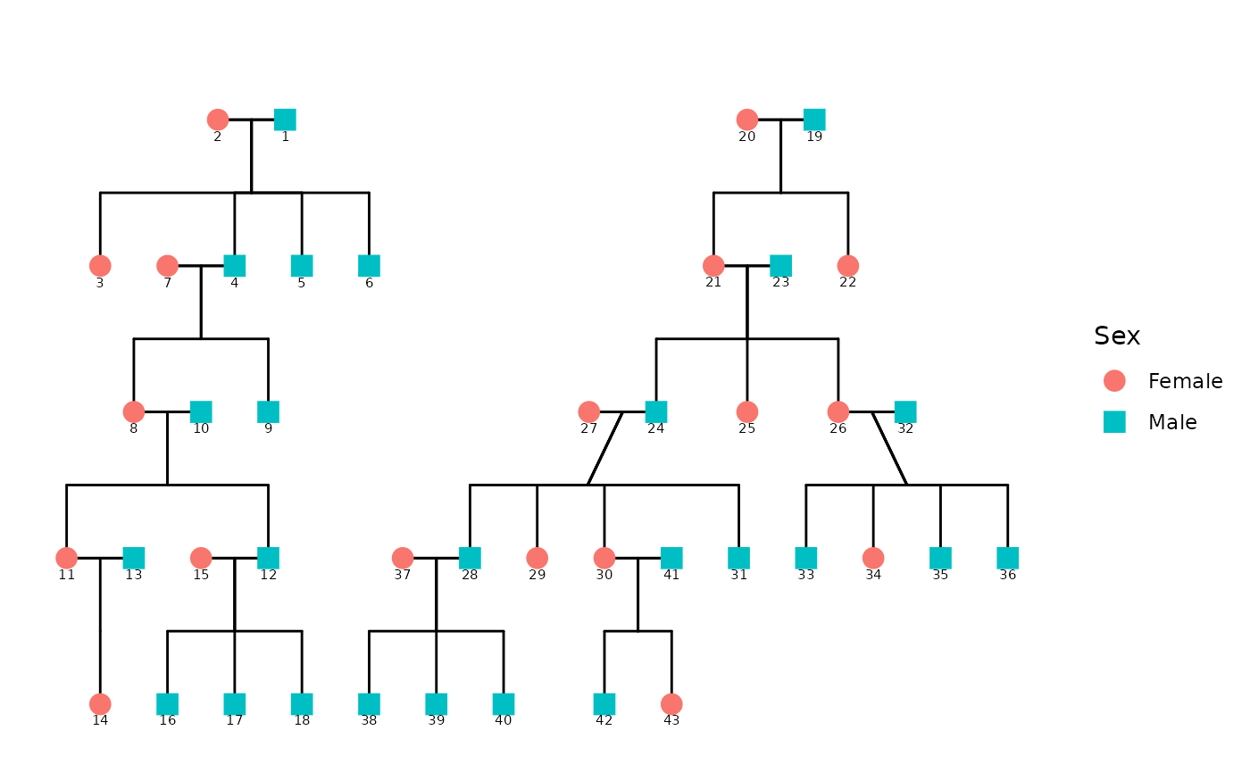
We compute the additive genetic relationship matrix using both the classic and partial parent methods. Because the pedigree is complete, we expect no differences in the resulting matrices.
ped_add_partial_complete <- ped2com(df,
  isChild_method = "partialparent",
  component = "additive",
  adjacency_method = "direct",
  sparse = FALSE
)
ped_add_classic_complete <- ped2com(df,
  isChild_method = "classic",
  component = "additive", adjacency_method = "direct",
  sparse = FALSE
)
The following plots display the full additive matrices. These matrices should be identical.
This can be confirmed visually and numerically.
library(ggpedigree)
ggRelatednessMatrix(as.matrix(ped_add_classic_complete),
  config =
    list(title = "Additive component - Classic method")
)
#> Warning in buildPlotConfig(default_config = default_config, config = config, :
#> The following config values are not recognized by getDefaultPlotConfig(): title
ggRelatednessMatrix(as.matrix(ped_add_partial_complete),
  config =
    list(title = "Additive component - Partial parent method")
)
#> Warning in buildPlotConfig(default_config = default_config, config = config, :
#> The following config values are not recognized by getDefaultPlotConfig(): title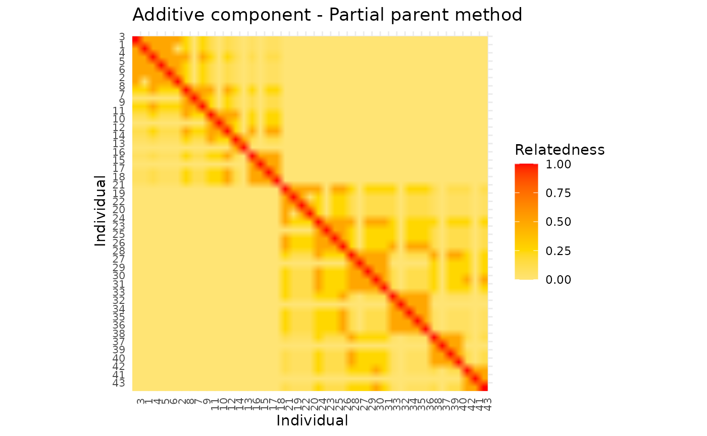
To verify this, we subtract one matrix from the other and calculate RMSE. The difference should be numerically zero. Indeed, it is 0.
library(corrplot)
#> corrplot 0.95 loaded
corrplot((as.matrix(ped_add_classic_complete) - as.matrix(ped_add_partial_complete)),
  method = "color", type = "lower", col.lim = c(0, 1),
  is.corr = FALSE, order = "hclust",
  tl.pos = "l", tl.col = "black", tl.srt = 5, tl.cex = 0.2,
  col = COL1("Reds", 100), mar = c(0, 0, 2, 0)
)
Introducing Missingness: Remove a Parent
To observe how the two methods diverge when data are incomplete, we remove one parent—starting with the mother of individual 4.
df$momID[df$ID == 4] <- NA
ped_add_partial_mom <- ped_add_partial <- ped2com(df,
  isChild_method = "partialparent",
  component = "additive",
  adjacency_method = "direct",
  sparse = FALSE
)

ped_add_classic_mom <- ped_add_classic <- ped2com(df,
  isChild_method = "classic",
  component = "additive", adjacency_method = "direct",
  sparse = FALSE
)
The two methods now treat individual 4 differently in the parent adjacency matrix. The classic method applies a fixed contribution because one parent remains. The partial parent method inflates the individual’s diagonal contribution to account for the missing parent.
The resulting additive matrices reflect this difference. The RMSE between the two matrices is 0.
corrplot(as.matrix(ped_add_classic),
  method = "color", type = "lower", col.lim = c(0, 1),
  is.corr = FALSE, title = "Classic (mother removed)",
  order = "hclust",
  tl.pos = "l", tl.col = "black", tl.srt = 5, tl.cex = 0.2,
  col = COL1("Reds", 100), mar = c(0, 0, 2, 0)
)
corrplot(as.matrix(ped_add_partial),
  method = "color", type = "lower", col.lim = c(0, 1),
  is.corr = FALSE, title = "Partial (mother removed)",
  order = "hclust",
  tl.pos = "l", tl.col = "black", tl.srt = 5, tl.cex = 0.2,
  col = COL1("Reds", 100), mar = c(0, 0, 2, 0)
)
We quantify the overall matrix difference:
Next, we compare each method to the matrix from the complete pedigree. This evaluates how much each method deviates from the correct additive structure.
corrplot(as.matrix(ped_add_classic_complete) - as.matrix(ped_add_classic),
  method = "color", type = "lower", col.lim = c(0, 1),
  is.corr = FALSE,
  order = "hclust",
  tl.pos = "l", tl.col = "black", tl.srt = 5, tl.cex = 0.2,
  col = COL1("Reds", 100), mar = c(0, 0, 2, 0)
)
#> Warning in corrplot(as.matrix(ped_add_classic_complete) -
#> as.matrix(ped_add_classic), : col.lim interval too wide, please set a suitable
#> value
The RMSE between the true additive component and the classic method is 0.
corrplot(as.matrix(ped_add_classic_complete - ped_add_partial),
  method = "color", type = "lower", col.lim = c(0, 1),
  is.corr = FALSE,
  order = "hclust",
  tl.pos = "l", tl.col = "black", tl.srt = 5, tl.cex = 0.2,
  col = COL1("Reds", 100), mar = c(0, 0, 2, 0)
)
#> Warning in corrplot(as.matrix(ped_add_classic_complete - ped_add_partial), :
#> col.lim interval too wide, please set a suitable value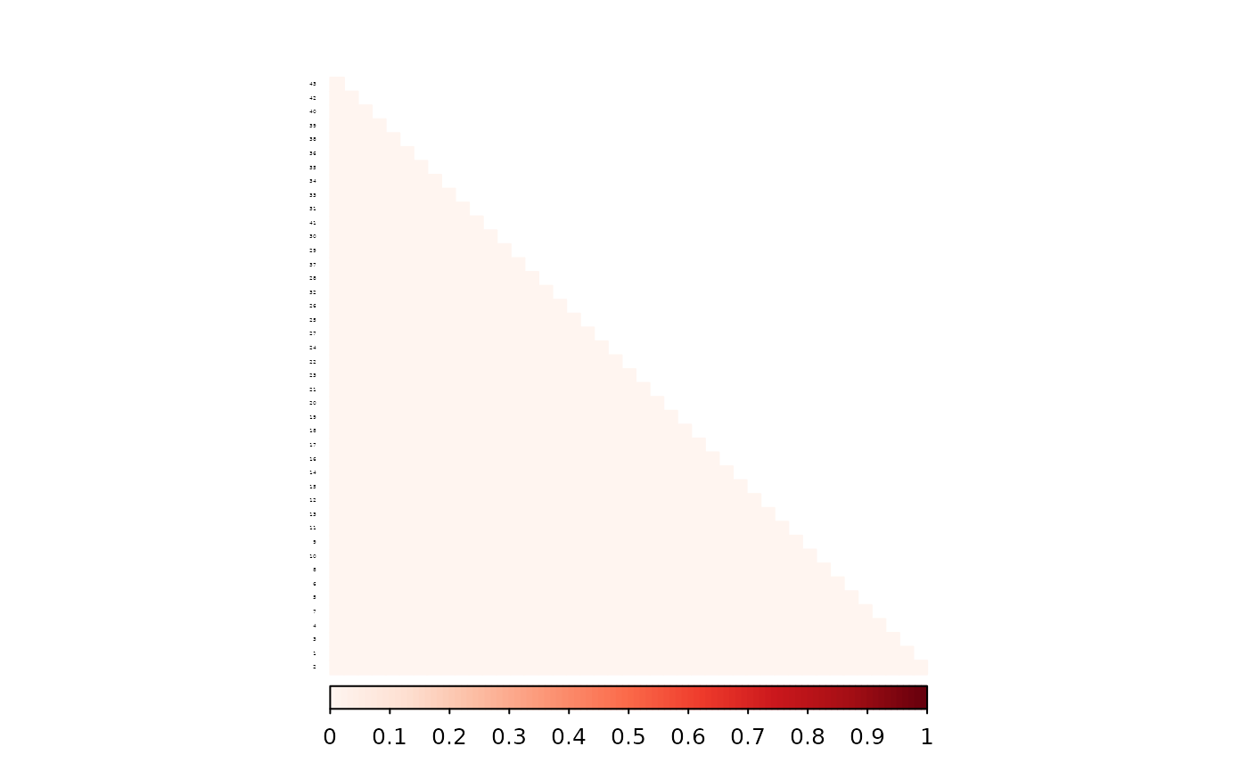
The RMSE between the true additive component and the partial parent method is 0.
The partial method shows smaller deviations from the complete matrix, confirming that it better preserves relatedness structure when one parent is missing.
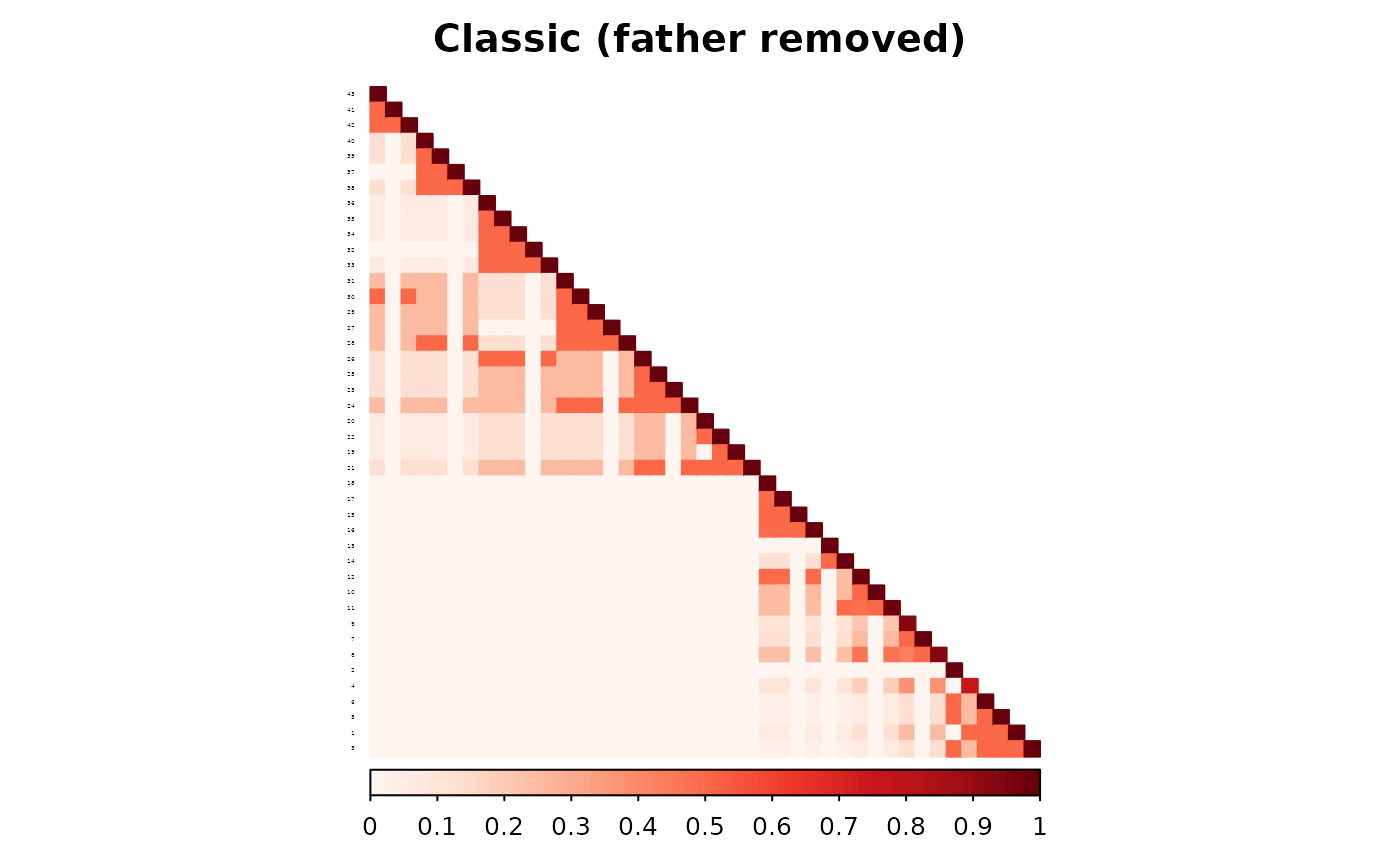
Removing the Father Instead
We now repeat the same process, this time removing the father of individual 4.
data(hazard)

df <- hazard # this is the data that we will use for the example


df$dadID[df$ID == 4] <- NA
# add
ped_add_partial_dad <- ped_add_partial <- ped2com(df,
  isChild_method = "partialparent",
  component = "additive",
  adjacency_method = "direct",
  sparse = FALSE
)

ped_add_classic_dad <- ped_add_classic <- ped2com(df,
  isChild_method = "classic",
  component = "additive", adjacency_method = "direct",
  sparse = FALSE
)
As we can see, the two matrices are different. The RMSE between the two matrices is 0.009811.
corrplot(as.matrix(ped_add_classic_dad),
  method = "color", type = "lower", col.lim = c(0, 1),
  is.corr = FALSE, title = "Classic (father removed)",
  order = "hclust",
  tl.pos = "l", tl.col = "black", tl.srt = 5, tl.cex = 0.2,
  col = COL1("Reds", 100), mar = c(0, 0, 2, 0)
)
corrplot(as.matrix(ped_add_partial_dad),
  method = "color", type = "lower", col.lim = c(0, 1),
  is.corr = FALSE, title = "Partial (father removed)",
  order = "hclust",
  tl.pos = "l", tl.col = "black", tl.srt = 5, tl.cex = 0.2,
  col = COL1("Reds", 100), mar = c(0, 0, 2, 0)
)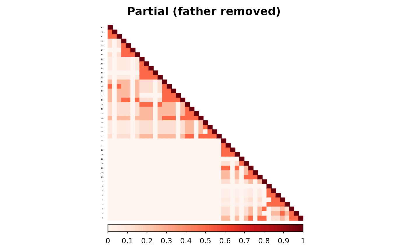
Again, we compare to the true matrix from the complete pedigree:
corrplot(as.matrix(ped_add_classic_complete - ped_add_classic),
  method = "color", type = "lower", col.lim = c(0, 1),
  is.corr = FALSE,
  order = "hclust",
  tl.pos = "l", tl.col = "black", tl.srt = 5, tl.cex = 0.2,
  col = COL1("Reds", 100), mar = c(0, 0, 2, 0)
)
corrplot(as.matrix(ped_add_classic_complete - ped_add_partial),
  method = "color", type = "lower", col.lim = c(0, 1),
  is.corr = FALSE,
  order = "hclust",
  tl.pos = "l", tl.col = "black", tl.srt = 5, tl.cex = 0.2,
  col = COL1("Reds", 100), mar = c(0, 0, 2, 0)
)
The partial parent method again yields a matrix closer to the full-data version.
Inbreeding Dataset: Family-Level Evaluation
To generalize the comparison across a larger and more varied set of
pedigrees, we use the inbreeding dataset. Each family in
this dataset is analyzed independently.
For each one, we construct the additive relationship matrix under complete information and then simulate two missingness scenarios:
Missing mother: One individual with a known mother is randomly selected, and the mother’s ID is set to NA.
Missing father: Similarly, one individual with a known father is selected, and the father’s ID is set to NA.
In each condition, we recompute the additive matrix using both the classic and partial parent methods. We then calculate the RMSE between each estimate and the matrix from the complete pedigree. This allows us to quantify which method more accurately reconstructs the original relatedness structure when parental data are partially missing.
inbreeding_list <- list()
results <- data.frame(
  famIDs = famIDs,
  RMSE_partial_dad = rep(NA, length(famIDs)),
  RMSE_partial_mom = rep(NA, length(famIDs)),
  RMSE_classic_dad = rep(NA, length(famIDs)),
  RMSE_classic_mom = rep(NA, length(famIDs)),
  max_R_classic_dad = rep(NA, length(famIDs)),
  max_R_partial_dad = rep(NA, length(famIDs)),
  max_R_classic_mom = rep(NA, length(famIDs)),
  max_R_partial_mom = rep(NA, length(famIDs)),
  max_R_classic = rep(NA, length(famIDs))
)
The loop below performs this procedure for all families in the dataset and stores both the RMSEs and the maximum relatedness values.
for (i in seq_len(famIDs)) {
  # make three versions to filter down
  df_fam_dad <- df_fam_mom <- df_fam <- df[df$famID == famIDs[i], ]

  results$RMSE_partial_mom[i] <- sqrt(mean((ped_add_classic_complete - ped_add_partial_mom)^2))


  ped_add_partial_complete <- ped2com(df_fam,
    isChild_method = "partialparent",
    component = "additive",
    adjacency_method = "direct",
    sparse = FALSE
  )

  ped_add_classic_complete <- ped2com(df_fam,
    isChild_method = "classic",
    component = "additive",
    adjacency_method = "direct",
    sparse = FALSE
  )


  # select first ID with a mom and dad
  momid_to_cut <- head(df_fam$ID[!is.na(df_fam$momID)], 1)
  dadid_to_cut <- head(df_fam$ID[!is.na(df_fam$dadID)], 1)

  df_fam_dad$dadID[df_fam$ID == dadid_to_cut] <- NA

  df_fam_mom$momID[df_fam$ID == momid_to_cut] <- NA

  ped_add_partial_dad <- ped2com(df_fam_dad,
    isChild_method = "partialparent",
    component = "additive",
    adjacency_method = "direct",
    sparse = FALSE
  )
  ped_add_classic_dad <- ped2com(df_fam_dad,
    isChild_method = "classic",
    component = "additive", adjacency_method = "direct",
    sparse = FALSE
  )

  results$RMSE_partial_dad[i] <- sqrt(mean((ped_add_classic_complete - ped_add_partial_dad)^2))
  results$RMSE_classic_dad[i] <- sqrt(mean((ped_add_classic_complete - ped_add_classic_dad)^2))
  results$max_R_classic_dad[i] <- max(as.matrix(ped_add_classic_dad))
  results$max_R_partial_dad[i] <- max(as.matrix(ped_add_partial_dad))


  ped_add_partial_mom <- ped2com(df_fam_mom,
    isChild_method = "partialparent",
    component = "additive",
    adjacency_method = "direct",
    sparse = FALSE
  )

  ped_add_classic_mom <- ped2com(df_fam_mom,
    isChild_method = "classic",
    component = "additive", adjacency_method = "direct",
    sparse = FALSE
  )

  results$RMSE_partial_mom[i] <- sqrt(mean((ped_add_classic_complete - ped_add_partial_mom)^2))
  results$RMSE_classic_mom[i] <- sqrt(mean((ped_add_classic_complete - ped_add_classic_mom)^2))
  results$max_R_classic_mom[i] <- max(as.matrix(ped_add_classic_mom))
  results$max_R_partial_mom[i] <- max(as.matrix(ped_add_partial_mom))
  results$max_R_classic[i] <- max(as.matrix(ped_add_classic_complete))

  inbreeding_list[[i]] <- list(
    df_fam = df_fam,
    ped_add_partial_complete = ped_add_partial_complete,
    ped_add_classic_complete = ped_add_classic_complete,
    ped_add_partial_dad = ped_add_partial_dad,
    ped_add_classic_dad = ped_add_classic_dad,
    ped_add_partial_mom = ped_add_partial_mom,
    ped_add_classic_mom = ped_add_classic_mom
  )
}
#> Warning in seq_len(famIDs): first element used of 'length.out' argument
Example: Family 1
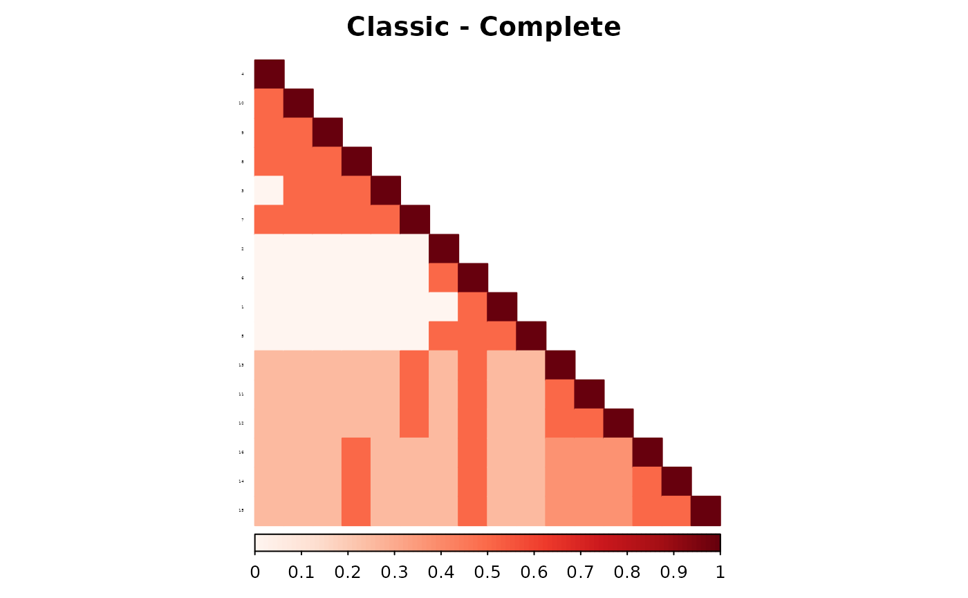
To understand what these matrices look like, we visualize them for one representative family. For this example, we select the first family in the dataset.

# pull the first family from the list
fam1 <- inbreeding_list[[1]]

corrplot(as.matrix(fam1$ped_add_classic_complete),
  method = "color", type = "lower", col.lim = c(0, 1),
  is.corr = FALSE, title = "Classic - Complete",
  order = "hclust",
  tl.pos = "l", tl.col = "black", tl.srt = 5, tl.cex = 0.2,
  col = COL1("Reds", 100), mar = c(0, 0, 2, 0)
)
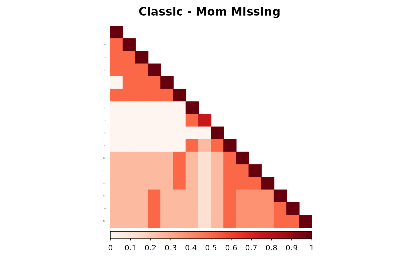
corrplot(as.matrix(fam1$ped_add_classic_mom),
  method = "color", type = "lower", col.lim = c(0, 1),
  is.corr = FALSE, title = "Classic - Mom Missing",
  order = "hclust",
  tl.pos = "l", tl.col = "black", tl.srt = 5, tl.cex = 0.2,
  col = COL1("Reds", 100), mar = c(0, 0, 2, 0)
)
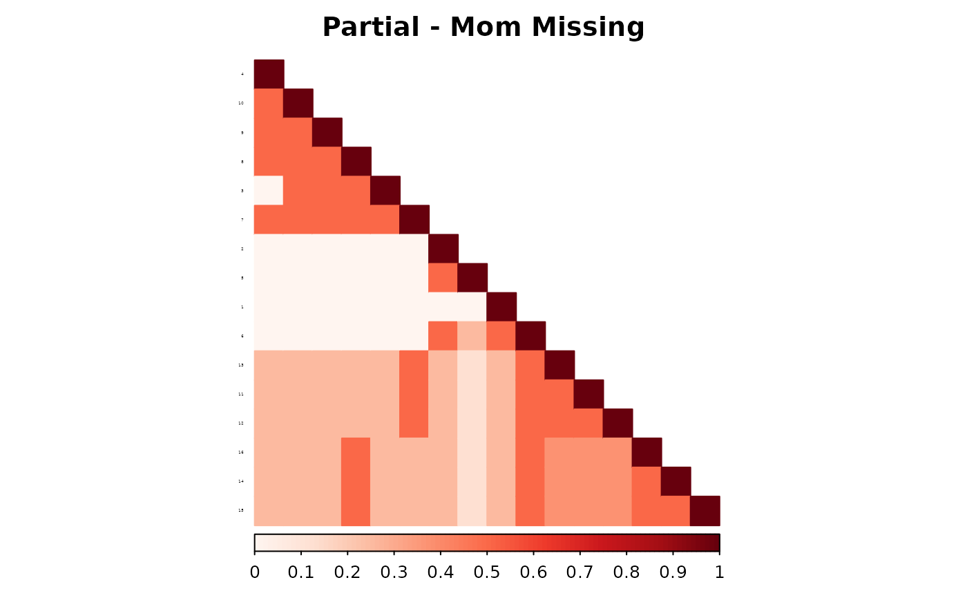
corrplot(as.matrix(fam1$ped_add_partial_mom),
  method = "color", type = "lower", col.lim = c(0, 1),
  is.corr = FALSE, title = "Partial - Mom Missing",
  order = "hclust",
  tl.pos = "l", tl.col = "black", tl.srt = 5, tl.cex = 0.2,
  col = COL1("Reds", 100), mar = c(0, 0, 2, 0)
)
corrplot(as.matrix(fam1$ped_add_classic_dad),
  method = "color", type = "lower", col.lim = c(0, 1),
  is.corr = FALSE, title = "Classic - Dad Missing",
  order = "hclust",
  tl.pos = "l", tl.col = "black", tl.srt = 5, tl.cex = 0.2,
  col = COL1("Reds", 100), mar = c(0, 0, 2, 0)
)
corrplot(as.matrix(fam1$ped_add_partial_dad),
  method = "color", type = "lower", col.lim = c(0, 1),
  is.corr = FALSE, title = "Partial - Dad Missing",
  order = "hclust",
  tl.pos = "l", tl.col = "black", tl.srt = 5, tl.cex = 0.2,
  col = COL1("Reds", 100), mar = c(0, 0, 2, 0)
)
To visualize the differences from the true matrix:
corrplot(as.matrix(fam1$ped_add_classic_complete - fam1$ped_add_classic_mom),
  method = "color", type = "lower", col.lim = c(0, 1),
  is.corr = FALSE, title = "Classic Mom Diff from Complete",
  order = "hclust",
  tl.pos = "l", tl.col = "black", tl.srt = 5, tl.cex = 0.2,
  col = COL1("Reds", 100), mar = c(0, 0, 2, 0)
)
corrplot(as.matrix(fam1$ped_add_classic_complete - fam1$ped_add_partial_mom),
  method = "color", type = "lower", col.lim = c(0, 1),
  is.corr = FALSE, title = "Partial Mom Diff from Complete",
  order = "hclust",
  tl.pos = "l", tl.col = "black", tl.srt = 5, tl.cex = 0.2,
  col = COL1("Reds", 100), mar = c(0, 0, 2, 0)
)
corrplot(as.matrix(fam1$ped_add_classic_complete - fam1$ped_add_classic_dad),
  method = "color", type = "lower", col.lim = c(0, 1),
  is.corr = FALSE, title = "Classic Dad Diff from Complete",
  order = "hclust",
  tl.pos = "l", tl.col = "black", tl.srt = 5, tl.cex = 0.2,
  col = COL1("Reds", 100), mar = c(0, 0, 2, 0)
)
corrplot(as.matrix(fam1$ped_add_classic_complete - fam1$ped_add_partial_dad),
  method = "color", type = "lower", col.lim = c(0, 1),
  is.corr = FALSE, title = "Partial Dad Diff from Complete",
  order = "hclust",
  tl.pos = "l", tl.col = "black", tl.srt = 5, tl.cex = 0.2,
  col = COL1("Reds", 100), mar = c(0, 0, 2, 0)
)
These plots show how each method responds to missing data, and whether it maintains consistency with the complete pedigree. We observe that the partial parent method typically introduces smaller deviations. If desired, this same diagnostic can be repeated for additional families, such as inbreeding_list[[2]].
Summary
Across all families in the inbreeding dataset, the results show a consistent pattern: the partial parent method outperforms the classic method in reconstructing the additive genetic relationship matrix when either a mother or a father is missing.
To make this explicit, we calculate the RMSE difference between methods. A positive value means that the partial method had lower RMSE (i.e., better accuracy) than the classic method:
results <- as.data.frame(results)

results$RMSE_diff_dad <- results$RMSE_classic_dad - results$RMSE_partial_dad
results$RMSE_diff_mom <- results$RMSE_classic_mom - results$RMSE_partial_mom
We can then summarize the pattern across families:
summary(dplyr::select(results, RMSE_diff_mom, RMSE_diff_dad))
#>  RMSE_diff_mom      RMSE_diff_dad
#>  Min.   :0.002127   Min.   :0.002127
#>  1st Qu.:0.002127   1st Qu.:0.002127
#>  Median :0.002127   Median :0.002127
#>  Mean   :0.002127   Mean   :0.002127
#>  3rd Qu.:0.002127   3rd Qu.:0.002127
#>  Max.   :0.002127   Max.   :0.002127
#>  NAs    :7          NAs    :7
In all families, both RMSE_diff_mom and
RMSE_diff_dad are positive—indicating that the classic
method produces larger the errors relative to the partial method. This
holds regardless of whether the missing parent is a mother or a
father.
To verify this directly:
mean(results$RMSE_diff_mom > 0, na.rm = TRUE)
#> [1] 1
mean(results$RMSE_diff_dad > 0, na.rm = TRUE)
#> [1] 1
These proportions show how often the partial method produces a lower RMSE across the dataset. This confirms the earlier findings: when pedigree data are incomplete, the partial parent method more faithfully reconstructs the full-data relatedness matrix.
results |>
  as.data.frame() |>
  dplyr::select(
    -famIDs, -RMSE_diff_mom, -RMSE_diff_dad, -max_R_classic_dad,
    -max_R_partial_dad, -max_R_classic_mom, -max_R_partial_mom, -max_R_classic
  ) |>
  summary()
#>  RMSE_partial_dad  RMSE_partial_mom  RMSE_classic_dad  RMSE_classic_mom
#>  Min.   :0.05634   Min.   :0.05634   Min.   :0.05846   Min.   :0.05846
#>  1st Qu.:0.05634   1st Qu.:0.05634   1st Qu.:0.05846   1st Qu.:0.05846
#>  Median :0.05634   Median :0.05634   Median :0.05846   Median :0.05846
#>  Mean   :0.05634   Mean   :0.05634   Mean   :0.05846   Mean   :0.05846
#>  3rd Qu.:0.05634   3rd Qu.:0.05634   3rd Qu.:0.05846   3rd Qu.:0.05846
#>  Max.   :0.05634   Max.   :0.05634   Max.   :0.05846   Max.   :0.05846
#>  NAs    :7         NAs    :7         NAs    :7         NAs    :7
This summary provides an overview of the RMSE values for each method across families. The advantage of the partial parent method in reconstructing relatedness was consistent when parental data are missing.