Adjacency matrix methods

Introduction

The ped2com function computes relationship matrices from pedigree data using a recursive algorithm based on parent-offspring connections. Central to this computation is the parent adjacency matrix, which defines how individuals in the pedigree are connected across generations. The adjacency matrix acts as the structural input from which genetic relatedness is propagated.

The function offers two methods for constructing this matrix:

The classic method, which assumes that all parents are known and that the adjacency matrix is complete.
The partial parent method, which allows for missing values in the parent adjacency matrix.

When parent data are complete, both methods return equivalent results. But when parental information is missing, their behavior diverges. This vignette illustrates how and why these differences emerge, and under what conditions the partial method provides more accurate results.

Hazard Data Example

We begin with the hazard dataset. First, we examine behavior under complete pedigree data.

library(BGmisc)

data(hazard)

df <- hazard # this is the data that we will use for the example

#> named list()

We compute the additive genetic relationship matrix using both the classic and partial parent methods. Because the pedigree is complete, we expect no differences in the resulting matrices.

ped_add_partial_complete <- ped2com(df,
  isChild_method = "partialparent",
  component = "additive",
  adjacency_method = "direct"
)
ped_add_classic_complete <- ped2com(df,
  isChild_method = "classic",
  component = "additive", adjacency_method = "direct"
)

The following plots display the full additive matrices. These matrices should be identical.

This can be confirmed visually and numerically.

library(corrplot)
#> corrplot 0.95 loaded


corrplot(as.matrix(ped_add_classic_complete),
  method = "color", type = "lower", col.lim = c(0, 1),
  is.corr = FALSE, title = "Additive component - Classic method"
)


corrplot(as.matrix(ped_add_partial_complete),
  method = "color", type = "lower", col.lim = c(0, 1),
  is.corr = FALSE, title = "Additive component - Partial parent method"
)

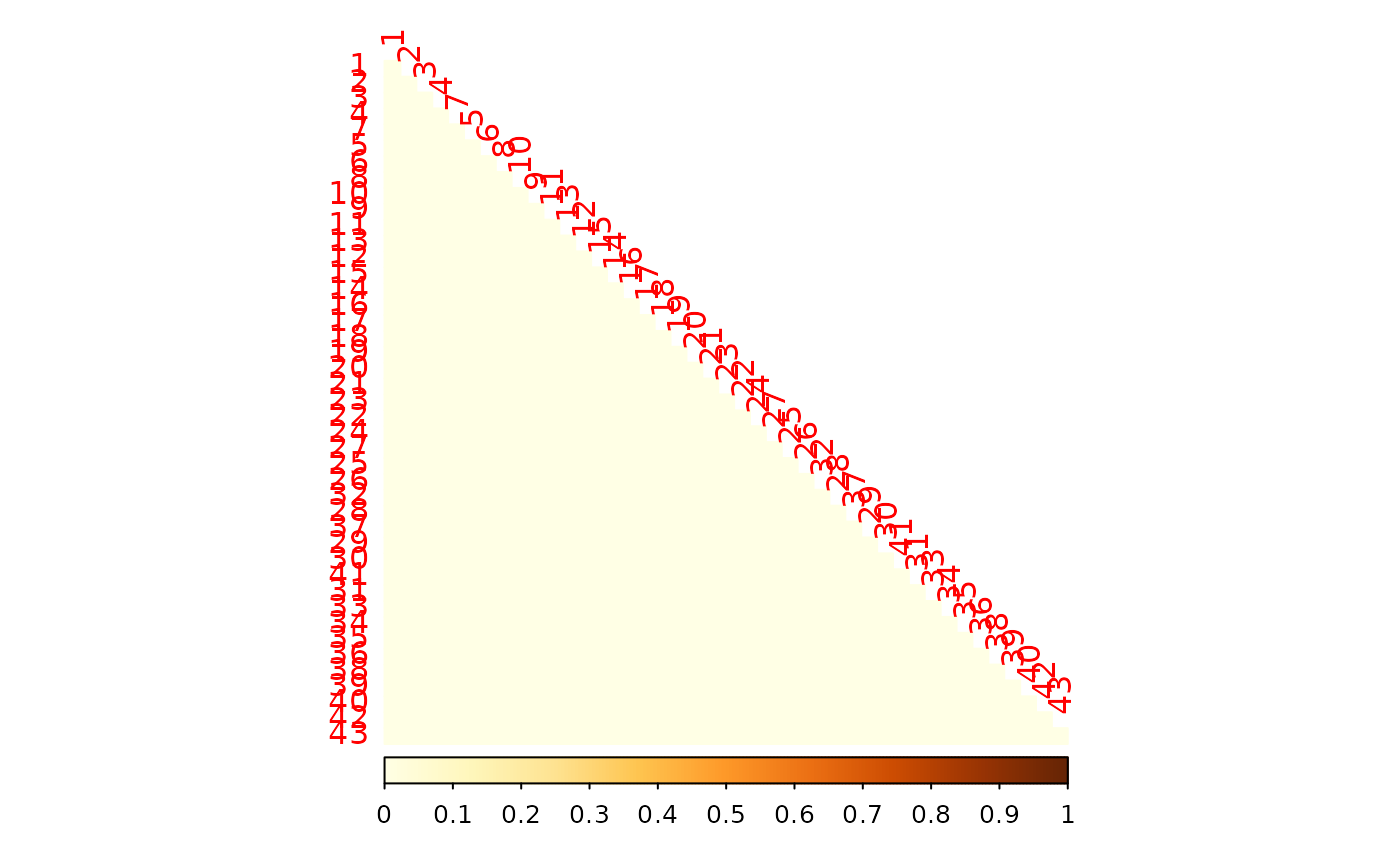
To verify this, we subtract one matrix from the other and calculate RMSE. The difference should be numerically zero. Indeed, it is NA.

corrplot(as.matrix(ped_add_classic_complete - ped_add_partial_complete),
  method = "color", type = "lower", col.lim = c(0, 1),
  is.corr = FALSE
)
#> Warning in corrplot(as.matrix(ped_add_classic_complete -
#> ped_add_partial_complete), : col.lim interval too wide, please set a suitable
#> value

Introducing Missingness: Remove a Parent

To observe how the two methods diverge when data are incomplete, we remove one parent—starting with the mother of individual 4.

df$momID[df$ID == 4] <- NA

ped_add_partial_mom <- ped_add_partial <- ped2com(df,
  isChild_method = "partialparent",
  component = "additive",
  adjacency_method = "direct"
)

ped_add_classic_mom <- ped_add_classic <- ped2com(df,
  isChild_method = "classic",
  component = "additive", adjacency_method = "direct"
)

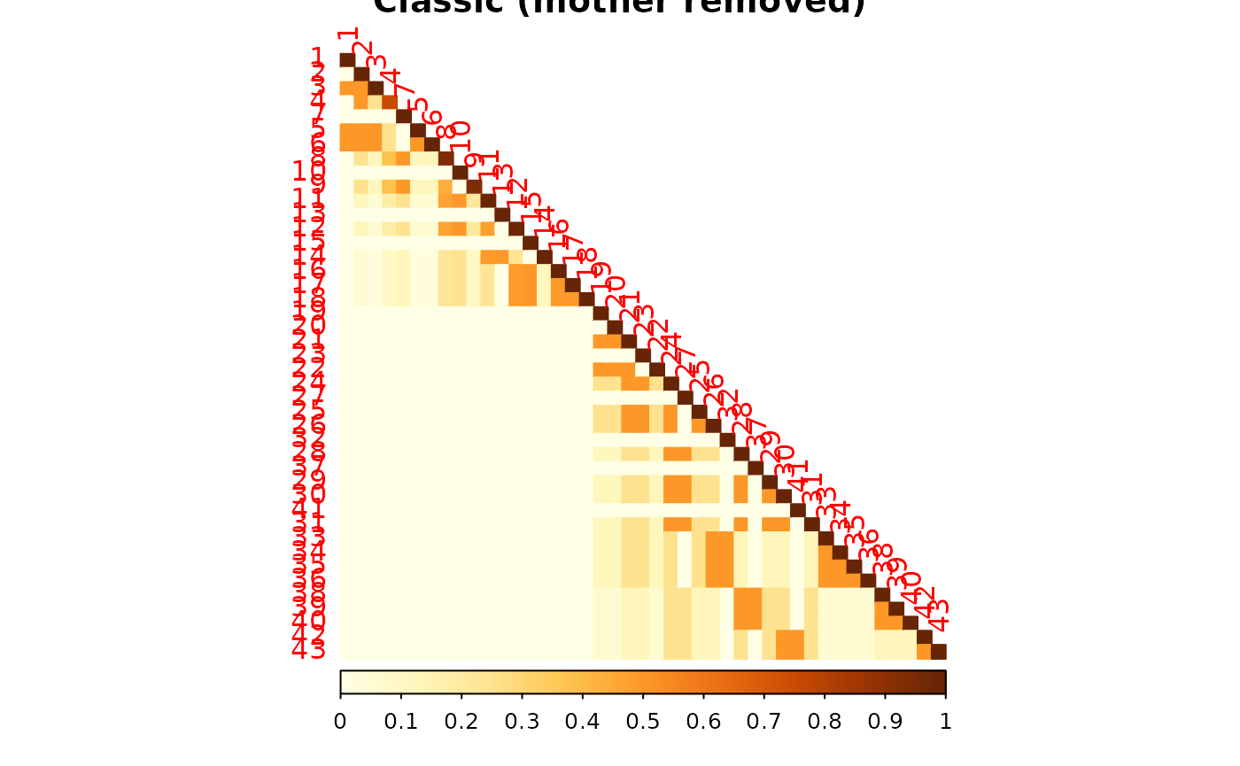
The two methods now treat individual 4 differently in the parent adjacency matrix. The classic method applies a fixed contribution because one parent remains. The partial parent method inflates the individual’s diagonal contribution to account for the missing parent.

The resulting additive matrices reflect this difference. The RMSE between the two matrices is NA.

corrplot(as.matrix(ped_add_classic),
  method = "color", type = "lower", col.lim = c(0, 1),
  is.corr = FALSE, title = "Classic (mother removed)"
)


corrplot(as.matrix(ped_add_partial),
  method = "color", type = "lower", col.lim = c(0, 1),
  is.corr = FALSE, title = "Partial (mother removed)"
)

We quantify the overall matrix difference:

sqrt(mean((ped_add_classic - ped_add_partial)^2))
#> Warning in mean.default((ped_add_classic - ped_add_partial)^2): argument is not
#> numeric or logical: returning NA
#> [1] NA

Next, we compare each method to the matrix from the complete pedigree. This evaluates how much each method deviates from the correct additive structure.

corrplot(as.matrix(ped_add_classic_complete - ped_add_classic),
  method = "color", type = "lower", col.lim = c(0, 1),
  is.corr = FALSE
)


sqrt(mean((ped_add_classic_complete - ped_add_classic)^2))
#> Warning in mean.default((ped_add_classic_complete - ped_add_classic)^2):
#> argument is not numeric or logical: returning NA
#> [1] NA

The RMSE between the true additive component and the classic method is NA.

corrplot(as.matrix(ped_add_classic_complete - ped_add_partial),
  method = "color", type = "lower", col.lim = c(0, 1),
  is.corr = FALSE
)


sqrt(mean((ped_add_classic_complete - ped_add_partial)^2))
#> Warning in mean.default((ped_add_classic_complete - ped_add_partial)^2):
#> argument is not numeric or logical: returning NA
#> [1] NA

The RMSE between the true additive component and the partial parent method is NA.

The partial method shows smaller deviations from the complete matrix, confirming that it better preserves relatedness structure when one parent is missing.

Removing the Father Instead

We now repeat the same process, this time removing the father of individual 4.

data(hazard)

df <- hazard # this is the data that we will use for the example


df$dadID[df$ID == 4] <- NA
# add
ped_add_partial_dad <- ped_add_partial <- ped2com(df,
  isChild_method = "partialparent",
  component = "additive",
  adjacency_method = "direct"
)

ped_add_classic_dad <- ped_add_classic <- ped2com(df,
  isChild_method = "classic",
  component = "additive", adjacency_method = "direct"
)

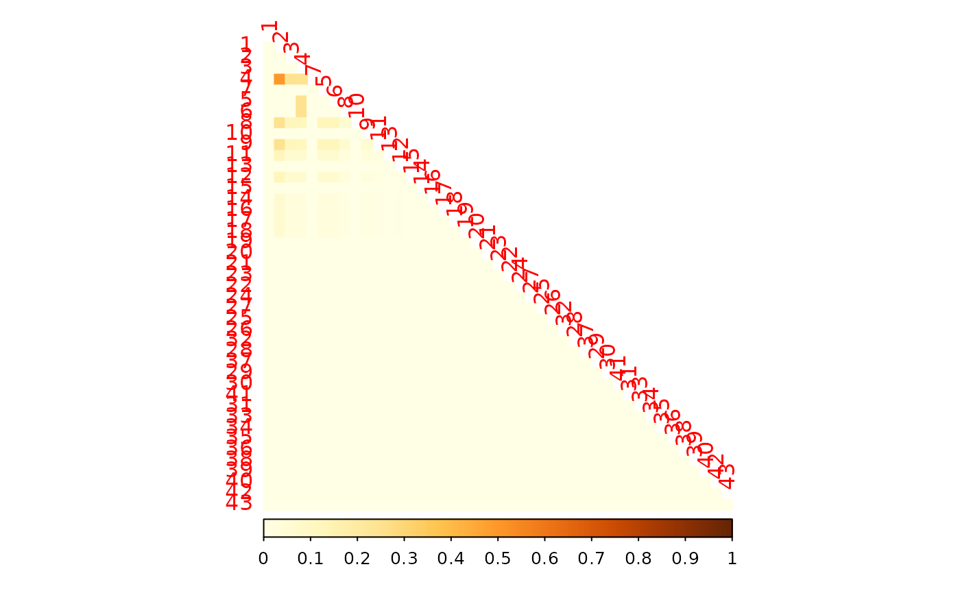
As we can see, the two matrices are different. The RMSE between the two matrices is NA.

corrplot(as.matrix(ped_add_classic_dad),
  method = "color", type = "lower", col.lim = c(0, 1),
  is.corr = FALSE, title = "Classic (father removed)"
)


corrplot(as.matrix(ped_add_partial_dad),
  method = "color", type = "lower", col.lim = c(0, 1),
  is.corr = FALSE, title = "Partial (father removed)"
)

Again, we compare to the true matrix from the complete pedigree:

corrplot(as.matrix(ped_add_classic_complete - ped_add_classic),
  method = "color", type = "lower", col.lim = c(0, 1),
  is.corr = FALSE
)


sqrt(mean((ped_add_classic_complete - ped_add_classic)^2))
#> Warning in mean.default((ped_add_classic_complete - ped_add_classic)^2):
#> argument is not numeric or logical: returning NA
#> [1] NA

corrplot(as.matrix(ped_add_classic_complete - ped_add_partial),
  method = "color", type = "lower", col.lim = c(0, 1),
  is.corr = FALSE
)


sqrt(mean((ped_add_classic_complete - ped_add_partial)^2))
#> Warning in mean.default((ped_add_classic_complete - ped_add_partial)^2):
#> argument is not numeric or logical: returning NA
#> [1] NA

The partial parent method again yields a matrix closer to the full-data version.

Inbreeding Dataset: Family-Level Evaluation

To generalize the comparison across a larger and more varied set of pedigrees, we use the inbreeding dataset. Each family in this dataset is analyzed independently.

data("inbreeding")

df <- inbreeding

FamIDs <- unique(df$FamID)

For each one, we construct the additive relationship matrix under complete information and then simulate two missingness scenarios:

Missing mother: One individual with a known mother is randomly selected, and the mother’s ID is set to NA.
Missing father: Similarly, one individual with a known father is selected, and the father’s ID is set to NA.

In each condition, we recompute the additive matrix using both the classic and partial parent methods. We then calculate the RMSE between each estimate and the matrix from the complete pedigree. This allows us to quantify which method more accurately reconstructs the original relatedness structure when parental data are partially missing.

inbreeding_list <- list()
results <- data.frame(
  FamIDs = FamIDs,
  RMSE_partial_dad = rep(NA, length(FamIDs)),
  RMSE_partial_mom = rep(NA, length(FamIDs)),
  RMSE_classic_dad = rep(NA, length(FamIDs)),
  RMSE_classic_mom = rep(NA, length(FamIDs)),
  max_R_classic_dad = rep(NA, length(FamIDs)),
  max_R_partial_dad = rep(NA, length(FamIDs)),
  max_R_classic_mom = rep(NA, length(FamIDs)),
  max_R_partial_mom = rep(NA, length(FamIDs)),
  max_R_classic = rep(NA, length(FamIDs))
)

The loop below performs this procedure for all families in the dataset and stores both the RMSEs and the maximum relatedness values.

for (i in 1:length(FamIDs)) {
  # make three versions to filter down
  df_fam_dad <- df_fam_mom <- df_fam <- df[df$FamID == FamIDs[i], ]

  results$RMSE_partial_mom[i] <- sqrt(mean((ped_add_classic_complete - ped_add_partial_mom)^2))


  ped_add_partial_complete <- ped2com(df_fam,
    isChild_method = "partialparent",
    component = "additive",
    adjacency_method = "direct"
  )

  ped_add_classic_complete <- ped2com(df_fam,
    isChild_method = "classic",
    component = "additive",
    adjacency_method = "direct"
  )


  # select first ID with a mom and dad
  momid_to_cut <- df_fam$ID[!is.na(df_fam$momID)] %>% head(1)
  dadid_to_cut <- df_fam$ID[!is.na(df_fam$dadID)] %>% head(1)

  df_fam_dad$dadID[df_fam$ID == dadid_to_cut] <- NA

  df_fam_mom$momID[df_fam$ID == momid_to_cut] <- NA

  ped_add_partial_dad <- ped2com(df_fam_dad,
    isChild_method = "partialparent",
    component = "additive",
    adjacency_method = "direct"
  )
  ped_add_classic_dad <- ped2com(df_fam_dad,
    isChild_method = "classic",
    component = "additive", adjacency_method = "direct"
  )

  results$RMSE_partial_dad[i] <- sqrt(mean((ped_add_classic_complete - ped_add_partial_dad)^2))
  results$RMSE_classic_dad[i] <- sqrt(mean((ped_add_classic_complete - ped_add_classic_dad)^2))
  results$max_R_classic_dad[i] <- max(as.matrix(ped_add_classic_dad))
  results$max_R_partial_dad[i] <- max(as.matrix(ped_add_partial_dad))


  ped_add_partial_mom <- ped2com(df_fam_mom,
    isChild_method = "partialparent",
    component = "additive",
    adjacency_method = "direct"
  )

  ped_add_classic_mom <- ped2com(df_fam_mom,
    isChild_method = "classic",
    component = "additive", adjacency_method = "direct"
  )

  results$RMSE_partial_mom[i] <- sqrt(mean((ped_add_classic_complete - ped_add_partial_mom)^2))
  results$RMSE_classic_mom[i] <- sqrt(mean((ped_add_classic_complete - ped_add_classic_mom)^2))
  results$max_R_classic_mom[i] <- max(as.matrix(ped_add_classic_mom))
  results$max_R_partial_mom[i] <- max(as.matrix(ped_add_partial_mom))
  results$max_R_classic[i] <- max(as.matrix(ped_add_classic_complete))

  inbreeding_list[[i]] <- list(
    df_fam = df_fam,
    ped_add_partial_complete = ped_add_partial_complete,
    ped_add_classic_complete = ped_add_classic_complete,
    ped_add_partial_dad = ped_add_partial_dad,
    ped_add_classic_dad = ped_add_classic_dad,
    ped_add_partial_mom = ped_add_partial_mom,
    ped_add_classic_mom = ped_add_classic_mom
  )
}
#> Warning in mean.default((ped_add_classic_complete - ped_add_partial_mom)^2):
#> argument is not numeric or logical: returning NA
#> Warning in mean.default((ped_add_classic_complete - ped_add_partial_dad)^2):
#> argument is not numeric or logical: returning NA
#> Warning in mean.default((ped_add_classic_complete - ped_add_classic_dad)^2):
#> argument is not numeric or logical: returning NA
#> Warning in mean.default((ped_add_classic_complete - ped_add_partial_mom)^2):
#> argument is not numeric or logical: returning NA
#> Warning in mean.default((ped_add_classic_complete - ped_add_classic_mom)^2):
#> argument is not numeric or logical: returning NA
#> Warning in mean.default((ped_add_classic_complete - ped_add_partial_mom)^2):
#> argument is not numeric or logical: returning NA
#> Warning in mean.default((ped_add_classic_complete - ped_add_partial_dad)^2):
#> argument is not numeric or logical: returning NA
#> Warning in mean.default((ped_add_classic_complete - ped_add_classic_dad)^2):
#> argument is not numeric or logical: returning NA
#> Warning in mean.default((ped_add_classic_complete - ped_add_partial_mom)^2):
#> argument is not numeric or logical: returning NA
#> Warning in mean.default((ped_add_classic_complete - ped_add_classic_mom)^2):
#> argument is not numeric or logical: returning NA
#> Warning in mean.default((ped_add_classic_complete - ped_add_partial_mom)^2):
#> argument is not numeric or logical: returning NA
#> Warning in mean.default((ped_add_classic_complete - ped_add_partial_dad)^2):
#> argument is not numeric or logical: returning NA
#> Warning in mean.default((ped_add_classic_complete - ped_add_classic_dad)^2):
#> argument is not numeric or logical: returning NA
#> Warning in mean.default((ped_add_classic_complete - ped_add_partial_mom)^2):
#> argument is not numeric or logical: returning NA
#> Warning in mean.default((ped_add_classic_complete - ped_add_classic_mom)^2):
#> argument is not numeric or logical: returning NA
#> Warning in mean.default((ped_add_classic_complete - ped_add_partial_mom)^2):
#> argument is not numeric or logical: returning NA
#> Warning in mean.default((ped_add_classic_complete - ped_add_partial_dad)^2):
#> argument is not numeric or logical: returning NA
#> Warning in mean.default((ped_add_classic_complete - ped_add_classic_dad)^2):
#> argument is not numeric or logical: returning NA
#> Warning in mean.default((ped_add_classic_complete - ped_add_partial_mom)^2):
#> argument is not numeric or logical: returning NA
#> Warning in mean.default((ped_add_classic_complete - ped_add_classic_mom)^2):
#> argument is not numeric or logical: returning NA
#> Warning in mean.default((ped_add_classic_complete - ped_add_partial_mom)^2):
#> argument is not numeric or logical: returning NA
#> Warning in mean.default((ped_add_classic_complete - ped_add_partial_dad)^2):
#> argument is not numeric or logical: returning NA
#> Warning in mean.default((ped_add_classic_complete - ped_add_classic_dad)^2):
#> argument is not numeric or logical: returning NA
#> Warning in mean.default((ped_add_classic_complete - ped_add_partial_mom)^2):
#> argument is not numeric or logical: returning NA
#> Warning in mean.default((ped_add_classic_complete - ped_add_classic_mom)^2):
#> argument is not numeric or logical: returning NA
#> Warning in mean.default((ped_add_classic_complete - ped_add_partial_mom)^2):
#> argument is not numeric or logical: returning NA
#> Warning in mean.default((ped_add_classic_complete - ped_add_partial_dad)^2):
#> argument is not numeric or logical: returning NA
#> Warning in mean.default((ped_add_classic_complete - ped_add_classic_dad)^2):
#> argument is not numeric or logical: returning NA
#> Warning in mean.default((ped_add_classic_complete - ped_add_partial_mom)^2):
#> argument is not numeric or logical: returning NA
#> Warning in mean.default((ped_add_classic_complete - ped_add_classic_mom)^2):
#> argument is not numeric or logical: returning NA
#> Warning in mean.default((ped_add_classic_complete - ped_add_partial_mom)^2):
#> argument is not numeric or logical: returning NA
#> Warning in mean.default((ped_add_classic_complete - ped_add_partial_dad)^2):
#> argument is not numeric or logical: returning NA
#> Warning in mean.default((ped_add_classic_complete - ped_add_classic_dad)^2):
#> argument is not numeric or logical: returning NA
#> Warning in mean.default((ped_add_classic_complete - ped_add_partial_mom)^2):
#> argument is not numeric or logical: returning NA
#> Warning in mean.default((ped_add_classic_complete - ped_add_classic_mom)^2):
#> argument is not numeric or logical: returning NA
#> Warning in mean.default((ped_add_classic_complete - ped_add_partial_mom)^2):
#> argument is not numeric or logical: returning NA
#> Warning in mean.default((ped_add_classic_complete - ped_add_partial_dad)^2):
#> argument is not numeric or logical: returning NA
#> Warning in mean.default((ped_add_classic_complete - ped_add_classic_dad)^2):
#> argument is not numeric or logical: returning NA
#> Warning in mean.default((ped_add_classic_complete - ped_add_partial_mom)^2):
#> argument is not numeric or logical: returning NA
#> Warning in mean.default((ped_add_classic_complete - ped_add_classic_mom)^2):
#> argument is not numeric or logical: returning NA

Example: Family `1`

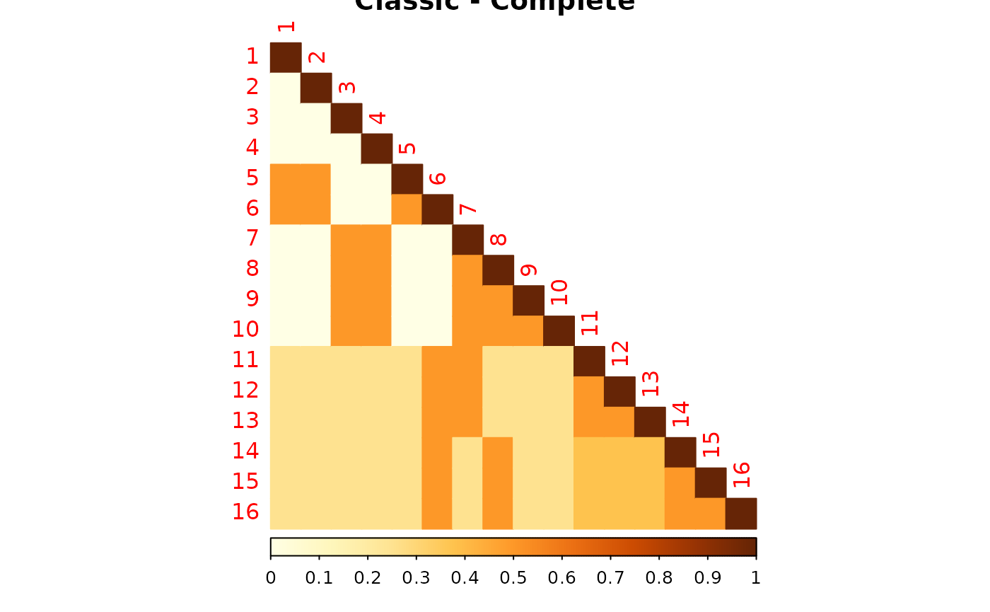
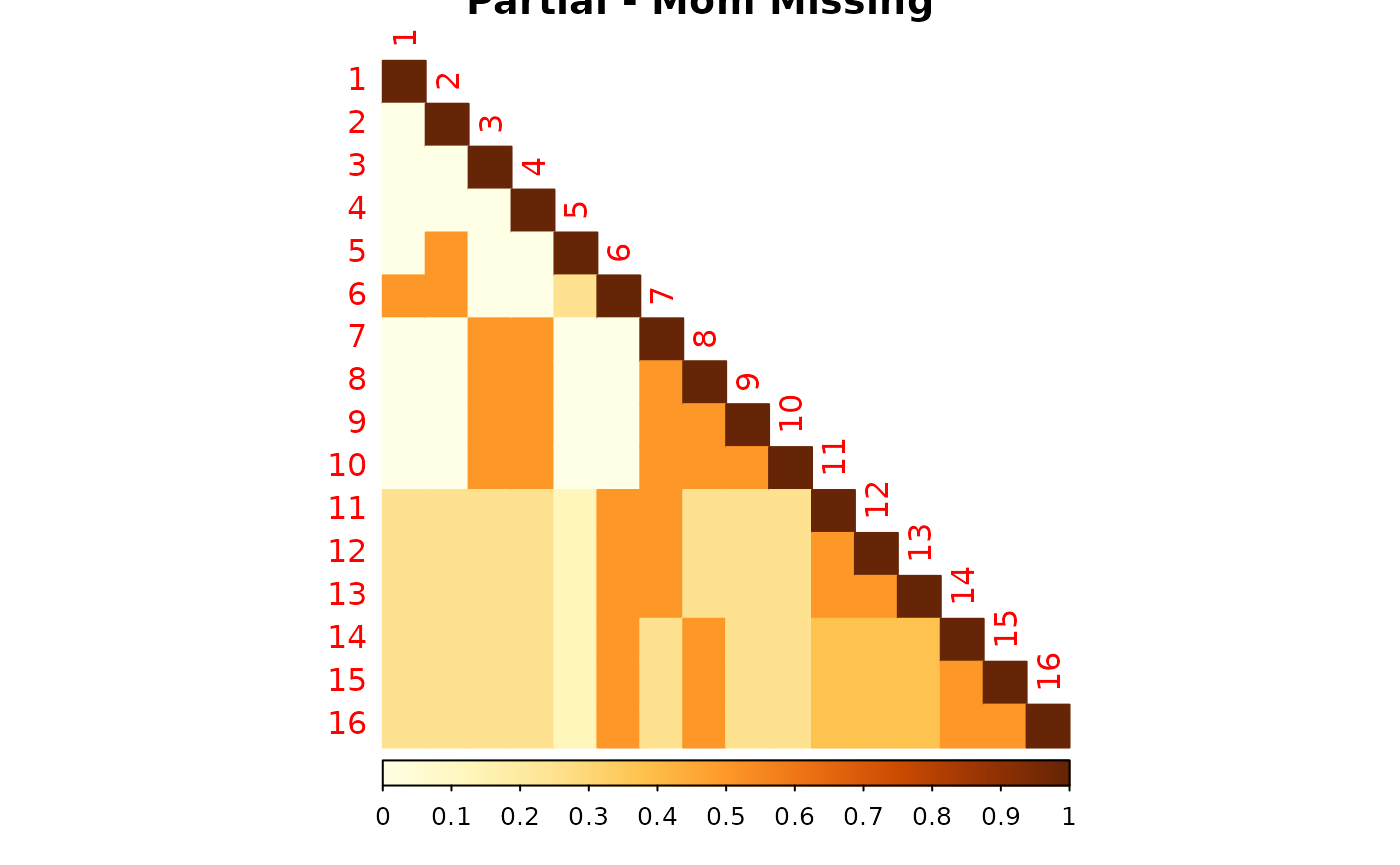
To understand what these matrices look like, we visualize them for one representative family. For this example, we select the first family in the dataset.

#> named list()

# pull the first family from the list
fam1 <- inbreeding_list[[1]]

corrplot(as.matrix(fam1$ped_add_classic_complete),
  method = "color", type = "lower", col.lim = c(0, 1),
  is.corr = FALSE, title = "Classic - Complete"
)


corrplot(as.matrix(fam1$ped_add_classic_mom),
  method = "color", type = "lower", col.lim = c(0, 1),
  is.corr = FALSE, title = "Classic - Mom Missing"
)


corrplot(as.matrix(fam1$ped_add_partial_mom),
  method = "color", type = "lower", col.lim = c(0, 1),
  is.corr = FALSE, title = "Partial - Mom Missing"
)


corrplot(as.matrix(fam1$ped_add_classic_dad),
  method = "color", type = "lower", col.lim = c(0, 1),
  is.corr = FALSE, title = "Classic - Dad Missing"
)


corrplot(as.matrix(fam1$ped_add_partial_dad),
  method = "color", type = "lower", col.lim = c(0, 1),
  is.corr = FALSE, title = "Partial - Dad Missing"
)

To visualize the differences from the true matrix:

corrplot(as.matrix(fam1$ped_add_classic_complete - fam1$ped_add_classic_mom),
  method = "color", type = "lower", col.lim = c(0, 1),
  is.corr = FALSE, title = "Classic Mom Diff from Complete"
)


corrplot(as.matrix(fam1$ped_add_classic_complete - fam1$ped_add_partial_mom),
  method = "color", type = "lower", col.lim = c(0, 1),
  is.corr = FALSE, title = "Partial Mom Diff from Complete"
)


corrplot(as.matrix(fam1$ped_add_classic_complete - fam1$ped_add_classic_dad),
  method = "color", type = "lower", col.lim = c(0, 1),
  is.corr = FALSE, title = "Classic Dad Diff from Complete"
)


corrplot(as.matrix(fam1$ped_add_classic_complete - fam1$ped_add_partial_dad),
  method = "color", type = "lower", col.lim = c(0, 1),
  is.corr = FALSE, title = "Partial Dad Diff from Complete"
)

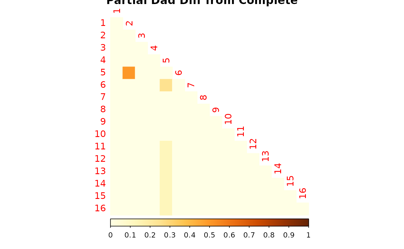
These plots show how each method responds to missing data, and whether it maintains consistency with the complete pedigree. We observe that the partial parent method typically introduces smaller deviations. If desired, this same diagnostic can be repeated for additional families, such as inbreeding_list[[2]].

Summary

Across all families in the inbreeding dataset, the results show a consistent pattern: the partial parent method outperforms the classic method in reconstructing the additive genetic relationship matrix when either a mother or a father is missing.

To make this explicit, we calculate the RMSE difference between methods. A positive value means that the partial method had lower RMSE (i.e., better accuracy) than the classic method:

results <- results %>%
  as.data.frame() %>%
  mutate(
    RMSE_diff_dad = RMSE_classic_dad - RMSE_partial_dad,
    RMSE_diff_mom = RMSE_classic_mom - RMSE_partial_mom
  )

We can then summarize the pattern across families:

results %>%
  select(RMSE_diff_mom, RMSE_diff_dad) %>%
  summary()
#>  RMSE_diff_mom RMSE_diff_dad
#>  Min.   : NA   Min.   : NA  
#>  1st Qu.: NA   1st Qu.: NA  
#>  Median : NA   Median : NA  
#>  Mean   :NaN   Mean   :NaN  
#>  3rd Qu.: NA   3rd Qu.: NA  
#>  Max.   : NA   Max.   : NA  
#>  NA's   :8     NA's   :8

In all families, both RMSE_diff_mom and RMSE_diff_dad are positive—indicating that the classic method produces larger the errors relative to the partial method. This holds regardless of whether the missing parent is a mother or a father.

To verify this directly:

mean(results$RMSE_diff_mom > 0, na.rm = TRUE)
#> [1] NaN
mean(results$RMSE_diff_dad > 0, na.rm = TRUE)
#> [1] NaN

These proportions show how often the partial method produces a lower RMSE across the dataset. This confirms the earlier findings: when pedigree data are incomplete, the partial parent method more faithfully reconstructs the full-data relatedness matrix.

results %>%
  as.data.frame() %>%
  select(
    -FamIDs, -RMSE_diff_mom, -RMSE_diff_dad, -max_R_classic_dad,
    -max_R_partial_dad, -max_R_classic_mom, -max_R_partial_mom, -max_R_classic
  ) %>%
  summary()
#>  RMSE_partial_dad RMSE_partial_mom RMSE_classic_dad RMSE_classic_mom
#>  Min.   : NA      Min.   : NA      Min.   : NA      Min.   : NA     
#>  1st Qu.: NA      1st Qu.: NA      1st Qu.: NA      1st Qu.: NA     
#>  Median : NA      Median : NA      Median : NA      Median : NA     
#>  Mean   :NaN      Mean   :NaN      Mean   :NaN      Mean   :NaN     
#>  3rd Qu.: NA      3rd Qu.: NA      3rd Qu.: NA      3rd Qu.: NA     
#>  Max.   : NA      Max.   : NA      Max.   : NA      Max.   : NA     
#>  NA's   :8        NA's   :8        NA's   :8        NA's   :8