What is a GEDCOM file?
GEDCOM (Genealogical Data Communication) is a plain-text file format used by virtually every genealogy platform — Ancestry, FamilySearch, MyHeritage, Gramps, and others.
A typical workflow looks like this:
- Build or find a family tree on Ancestry.com (or similar).
- Export it as a
.gedfile from the tree settings page. - Load it into R with
readGedcom().
The file itself is a structured text file.
Here is a small slice:
0 @I1@ INDI
1 NAME William Pitt /Waugh/
1 SEX M
1 BIRT
2 DATE 28 APR 1775
2 PLAC Adams County, Pennsylvania, USA
1 DEAT
2 DATE 14 AUG 1852
2 PLAC Wilkes County, North Carolina, USA
1 FAMS @F28@
1 FAMS @F29@

0 @F28@ FAM
1 HUSB @I1@
1 WIFE @I2@
1 CHIL @I3@

0 @F29@ FAM
1 HUSB @I1@
1 WIFE @I4@
1 CHIL @I5@
Individual records (INDI) hold person-level information;
family records (FAM) link spouses and children and carry
marriage or divorce events.
Why use R for genealogy?
The tidygedcom package provides tools for parsing and tidying GEDCOM files, making it easier to work with genealogical data in R. R’s powerful data manipulation capabilities allow researchers to clean, analyze, and visualize genealogical data in ways that may not be possible with traditional genealogy software. Additionally, R’s extensive ecosystem of packages for statistical analysis and machine learning can be applied to genealogical data to uncover patterns and insights that may not be immediately apparent.
Exporting your own GEDCOM file
Before you can analyze a tree, you need to get it out of whatever platform you built it on. The details differ by service, but the shape of the process is the same everywhere: find the tree’s settings page, request an export, wait for the file to be generated, and download it. Below is the process on Ancestry.com, which is where the example tree used throughout these vignettes came from.
Start from your tree’s settings page. Each tree has its own URL of
the form
https://www.ancestry.com/family-tree/tree/<TREE_ID>/settings/info,
reachable from the tree page itself.
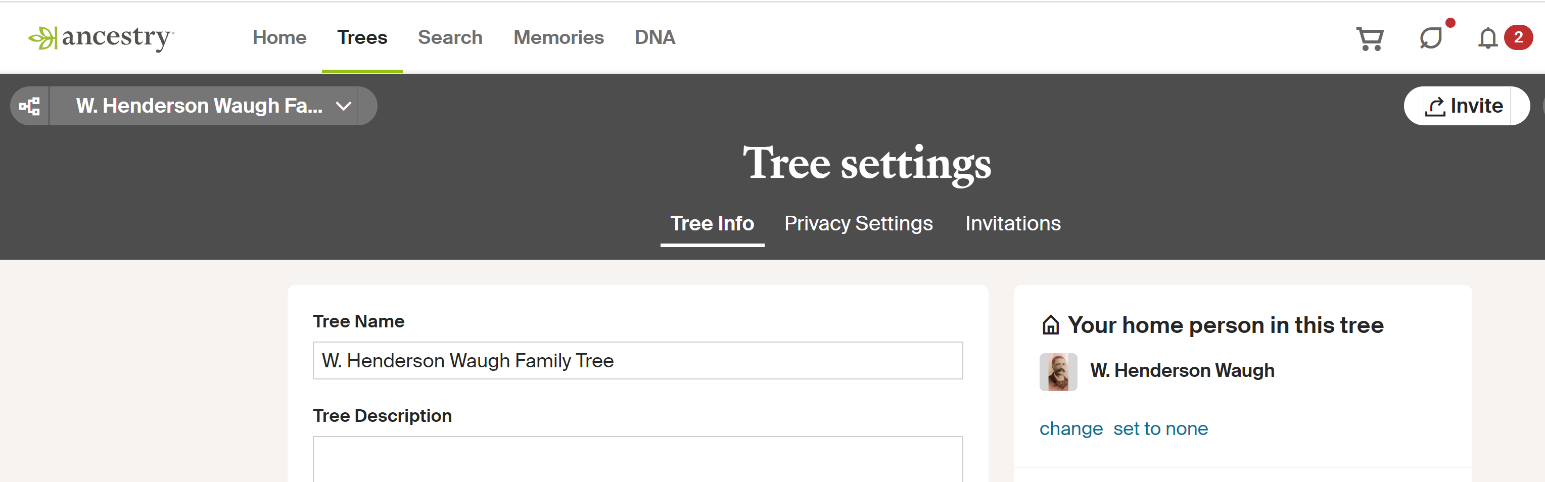
Scroll down and you will find the export option.
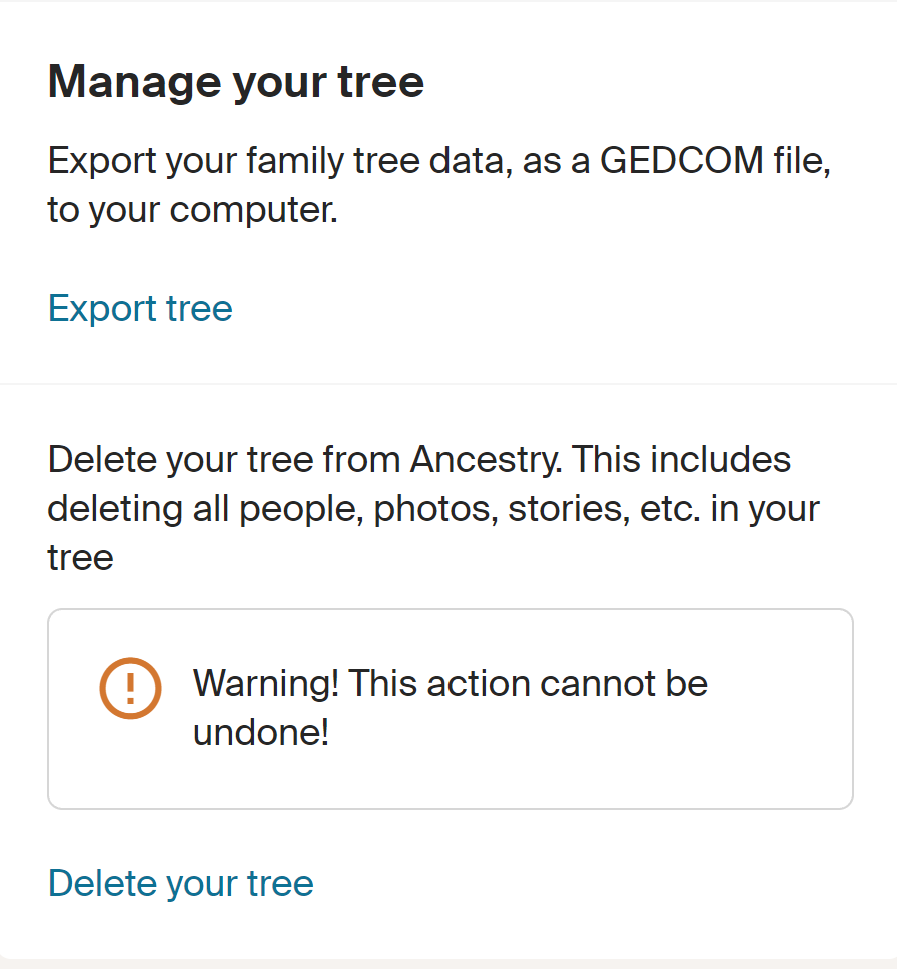
Selecting it opens a confirmation dialog.
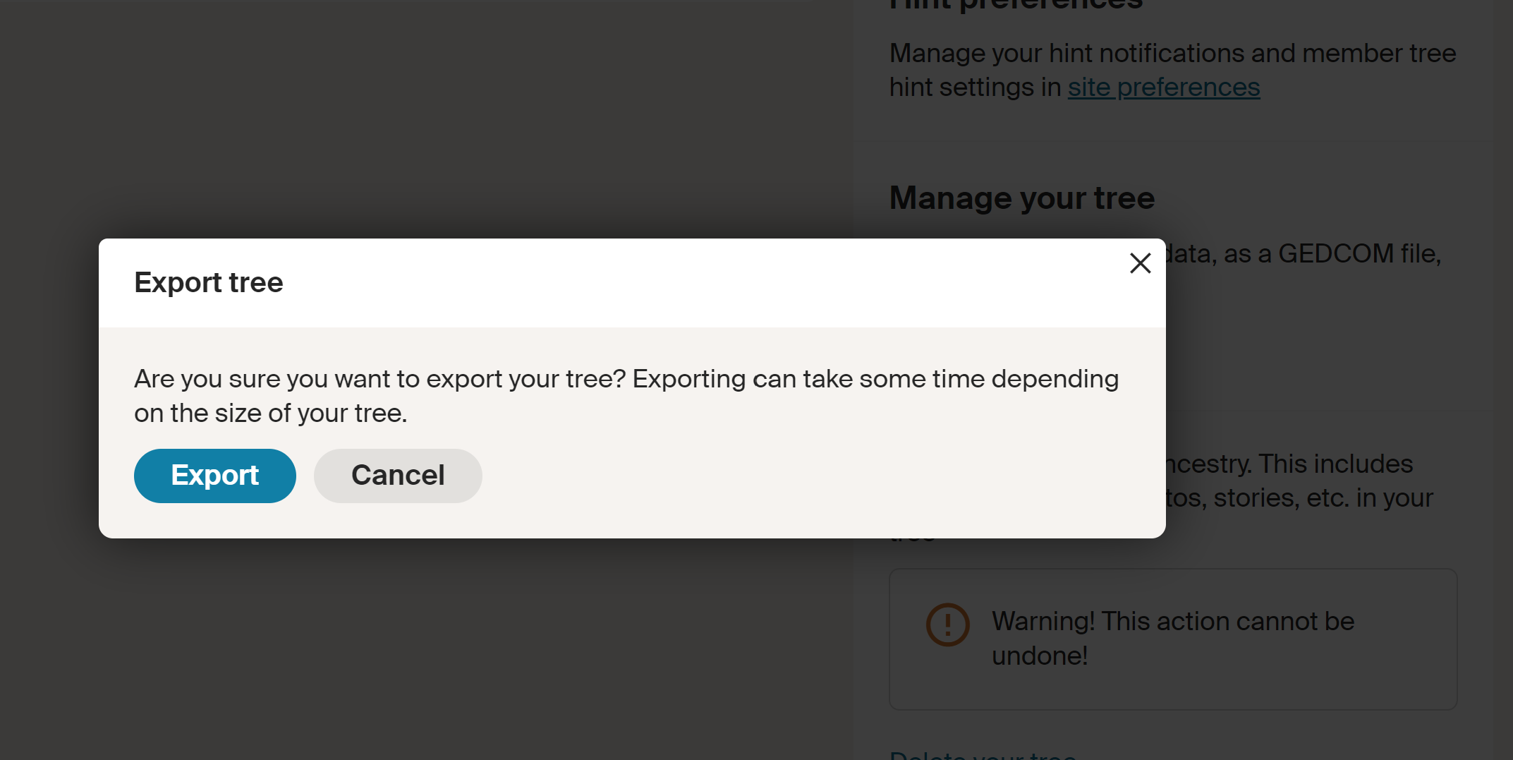
Once confirmed, the service builds a GEDCOM file from the current state of your tree. A small tree finishes in a few seconds; trees with several thousand people can take noticeably longer. When it is ready, you can download it as a zip archive.
Two things are worth knowing before you write any analysis code against the result.
Person IDs are not stable across exports. The file is generated fresh each time, and the identifiers assigned to individuals may differ between two exports of the same tree. Never hard-code an ID. Locate people by name, by birth date, or by some other durable attribute:
# Fragile -- the ID may change with the next export
henderson_id <- 242766628698

# Durable -- locate the person by a fact about them
henderson_id <- ped$personID[grepl("W. Henderson Waugh", ped$name)]
The export arrives zipped. You can unzip it by hand, or from R, which keeps the whole pipeline reproducible:
unzip("My Family Tree.zip", overwrite = TRUE)

ped <- readGedcom("My Family Tree.ged", verbose = FALSE)
It is worth peeking at the raw text before parsing, both to confirm the file is what you expect and to get a feel for how your particular platform writes its records:
raw_ged <- readLines("My Family Tree.ged")
head(raw_ged, 15)

# Jump to a specific person to see how their facts are recorded
line_num <- which(grepl("1 NAME W. Henderson /Waugh/", raw_ged, fixed = TRUE))
raw_ged[line_num:(line_num + 20)]
A word on privacy: an export of a living person’s tree contains birth
dates, places, and relationships for living people. Think carefully
before committing a .ged file to a public repository or
sharing it alongside a publication. The example files shipped with this
package deliberately contain only individuals who died before 1965.
A minimal example
This vignette uses a real family tree as its running example: the W. Henderson Waugh Family Tree. We’ll discuss more about our running example in another vignette. (But briefly, the Waugh family tree is a genetic genealogy collaboration between two Wake Forest psychology faculty – SMG and CEW. See Griffin (2017) for more on the historical context of the Waugh family tree.) The tidygedcom package provides the tools for parsing and tidying GEDCOM files, and the Waugh family tree provides a real-world test case for these tools.
We construct a small GEDCOM in memory that captures the key relationships described above.
This allows all code examples below to run without an external file.
sample_ged <- c(
  "0 HEAD",
  "1 GEDC",
  "2 VERS 5.5.1",
  "1 CHAR UTF-8",

  # William Pitt Waugh Sr. — the common paternal ancestor
  "0 @I1@ INDI",
  "1 NAME William Pitt /Waugh/",
  "1 SEX M",
  "1 BIRT",
  "2 DATE 28 APR 1775",
  "2 PLAC Adams County, Pennsylvania, USA",
  "1 DEAT",
  "2 DATE 14 AUG 1852",
  "2 PLAC Wilkes County, North Carolina, USA",
  "1 FAMS @F1@",
  "1 FAMS @F2@",

  # Matilda Grinton — mother of W. Henderson Waugh
  "0 @I2@ INDI",
  "1 NAME Matilda /Grinton/",
  "1 SEX F",
  "1 BIRT",
  "2 DATE ABT 1797",
  "2 PLAC North Carolina, USA",
  "1 FAMS @F1@",

  # W. Henderson Waugh — 2nd great-grandfather of focal person
  "0 @I3@ INDI",
  "1 NAME W. Henderson /Waugh/",
  "1 SEX M",
  "1 BIRT",
  "2 DATE ABT 1835",
  "2 PLAC Wilkes County, North Carolina, USA",
  "1 FAMC @F1@",
  "1 FAMS @F3@",

  # Martha Law Segraves — mother of William Pitt Waugh Jr.
  "0 @I4@ INDI",
  "1 NAME Martha Law /Segraves/",
  "1 SEX F",
  "1 BIRT",
  "2 DATE OCT 1814",
  "1 FAMS @F2@",

  # William Pitt Waugh Jr. (born William Segraves) — paternal half-brother of W. Henderson
  "0 @I5@ INDI",
  "1 NAME William Pitt /Waugh/ Jr.",
  "1 SEX M",
  "1 BIRT",
  "2 DATE 1844",
  "2 PLAC Wilkes County, North Carolina, USA",
  "1 DEAT",
  "2 DATE FEB 1880",
  "1 FAMC @F2@",
  "1 FAMS @F4@",

  # Laura Watkins — wife of W. Henderson Waugh
  "0 @I6@ INDI",
  "1 NAME Laura /Watkins/",
  "1 SEX F",
  "1 BIRT",
  "2 DATE ABT 1846",
  "2 PLAC North Carolina, USA",
  "1 FAMS @F3@",

  # John William (Bud) Waugh — son of W. Henderson; great-grandfather of focal person
  "0 @I7@ INDI",
  "1 NAME John William /Waugh/",
  "1 SEX M",
  "1 BIRT",
  "2 DATE ABT JUN 1880",
  "2 PLAC North Carolina, USA",
  "1 FAMC @F3@",

  # James Monroe Waugh — son of William Pitt Jr.; Y-DNA candidate branch
  "0 @I8@ INDI",
  "1 NAME James Monroe /Waugh/",
  "1 SEX M",
  "1 BIRT",
  "2 DATE 10 NOV 1867",
  "1 DEAT",
  "2 DATE 23 JUL 1937",
  "1 FAMC @F4@",

  # Family 1: William Pitt Sr. + Matilda Grinton -> W. Henderson Waugh
  "0 @F1@ FAM",
  "1 HUSB @I1@",
  "1 WIFE @I2@",
  "1 CHIL @I3@",

  # Family 2: William Pitt Sr. + Martha Segraves -> William Pitt Jr.
  # _SREL friend marks this as a non-marital relationship in Ancestry exports
  "0 @F2@ FAM",
  "1 HUSB @I1@",
  "1 WIFE @I4@",
  "1 CHIL @I5@",
  "1 _SREL friend",

  # Family 3: W. Henderson Waugh + Laura Watkins
  "0 @F3@ FAM",
  "1 HUSB @I3@",
  "1 WIFE @I6@",
  "1 CHIL @I7@",
  "1 MARR",
  "2 DATE 24 JUN 1877",
  "2 PLAC Wilkes County, North Carolina, USA",

  # Family 4: William Pitt Jr. + wife
  "0 @F4@ FAM",
  "1 HUSB @I5@",
  "1 CHIL @I8@",
  "0 TRLR"
)

tmp_ged <- tempfile(fileext = ".ged")
writeLines(sample_ged, tmp_ged)
Reading individual records: readGedcom()
readGedcom() parses all INDI blocks and
returns one row per person. It infers momID and
dadID automatically by tracing FAMC →
FAMS links — no manual ID mapping required.
ped <- readGedcom(tmp_ged, verbose = FALSE)
ped[, c("personID", "name", "sex", "birth_date", "death_date", "momID", "dadID")]
#>   personID                   name sex   birth_date  death_date momID dadID
#> 1        1     William Pitt Waugh   M  28 APR 1775 14 AUG 1852  <NA>  <NA>
#> 2        2        Matilda Grinton   F     ABT 1797        <NA>  <NA>  <NA>
#> 3        3     W. Henderson Waugh   M     ABT 1835        <NA>     2     1
#> 4        4    Martha Law Segraves   F     OCT 1814        <NA>  <NA>  <NA>
#> 5        5 William Pitt Waugh Jr.   M         1844    FEB 1880     4     1
#> 6        6          Laura Watkins   F     ABT 1846        <NA>  <NA>  <NA>
#> 7        7     John William Waugh   M ABT JUN 1880        <NA>     6     3
#> 8        8     James Monroe Waugh   M  10 NOV 1867 23 JUL 1937  <NA>     5
Notice that W. Henderson Waugh and William Pitt Waugh Jr. share the
same dadID — William Pitt Waugh Sr. — reflecting the
half-sibling relationship in the parsed data.
GEDCOM version
attr(ped, "gedcom_version")
#> [1] "5.5.1"
Quick overview: summarizeGedcom()
summarizeGedcom(ped)
#> GEDCOM Summary  (version: 5.5.1 )
#>   Individuals: 8
#>   Sex: M = 5 | F = 3 | Unknown = 0
#>   With birth date: 8  (100%)
#>   With death date: 3  (38%)
#>   With birth place: 6  (75%)
#>   With death place: 1  (12%)
#>   With known mother: 3  (38%)
#>   With known father: 4  (50%)
For a large real-world file (the full W. Henderson Waugh tree has several hundred individuals), this is the first thing to call after loading — it shows at a glance how much birth, death, and parentage data is present before any cleaning.
Working with dates
GEDCOM dates are raw strings that often carry qualifiers
(ABT, BEF, AFT) or calendar
escape codes (@#DGREGORIAN@). Historical genealogy —
especially for antebellum American records — is full of approximate
dates: birth years reconstructed from census age questions, death years
inferred from probate filings, and marriage dates from county clerk
records that were never systematically kept.
Parse to Date objects
Pass parse_dates = TRUE to convert
birth_date and death_date to proper
Date objects. Qualifiers (ABT,
AFT, BEF, BET, in both the
specification’s ABT form and Ancestry’s Abt.
form) and calendar escapes are stripped first:
ped_dates <- readGedcom(tmp_ged, parse_dates = TRUE, verbose = FALSE)
ped_dates[, c("name", "birth_date", "death_date")]
#>                     name birth_date death_date
#> 1     William Pitt Waugh 1775-04-28 1852-08-14
#> 2        Matilda Grinton 1797-06-15       <NA>
#> 3     W. Henderson Waugh 1835-06-15       <NA>
#> 4    Martha Law Segraves 1814-10-15       <NA>
#> 5 William Pitt Waugh Jr. 1844-06-15 1880-02-15
#> 6          Laura Watkins 1846-06-15       <NA>
#> 7     John William Waugh 1880-06-15       <NA>
#> 8     James Monroe Waugh 1867-11-10 1937-07-23
A Date needs a day, but historical records frequently
supply only a month or only a year. Rather than discard those dates,
readGedcom() completes them with the midpoint of the
interval that is known: the 15th of a known month, and 15 June
for a known year. "Oct 1814" becomes
1814-10-15, and "abt 1835" becomes
1835-06-15. Midpoints are used because they minimize the
expected distance from the true date.
This matters more than it might sound. In this small sample, five of the eight birth dates carry no day component — for antebellum records reconstructed from census age questions, partial dates are the norm rather than the exception, and dropping them would discard most of the data.
The imputed precision is not real, though, and you should not present
it as if it were. When you need to know which dates were exact, set
impute_partial_dates = FALSE to keep only dates that
specify a day, or read the file twice and compare:
exact <- readGedcom(tmp_ged,
  parse_dates = TRUE,
  impute_partial_dates = FALSE, verbose = FALSE
)

data.frame(
  name = ped_dates$name,
  birth = ped_dates$birth_date,
  was_exact = !is.na(exact$birth_date)
)
#>                     name      birth was_exact
#> 1     William Pitt Waugh 1775-04-28      TRUE
#> 2        Matilda Grinton 1797-06-15     FALSE
#> 3     W. Henderson Waugh 1835-06-15     FALSE
#> 4    Martha Law Segraves 1814-10-15     FALSE
#> 5 William Pitt Waugh Jr. 1844-06-15     FALSE
#> 6          Laura Watkins 1846-06-15     FALSE
#> 7     John William Waugh 1880-06-15     FALSE
#> 8     James Monroe Waugh 1867-11-10      TRUE
Extract a year from any GEDCOM date string
Not all dates parse cleanly to Date objects —
"ABT 1835" or "OCT 1814" have no day
component. extractGedcomYear() handles all forms and
returns an integer year:
dates_raw <- c(
  "28 APR 1775", "14 AUG 1852", "ABT 1835", "OCT 1814",
  "1844", "ABT JUN 1880", NA
)
extractGedcomYear(dates_raw)
#> [1] 1775 1852 1835 1814 1844 1880   NA
A typical use: add a birth_year column robust to
approximate dates, then flag individuals who may still be living:
ped$birth_year <- extractGedcomYear(ped$birth_date)
ped$death_year <- extractGedcomYear(ped$death_date)
ped[, c("name", "birth_year", "death_year")]
#>                     name birth_year death_year
#> 1     William Pitt Waugh       1775       1852
#> 2        Matilda Grinton       1797         NA
#> 3     W. Henderson Waugh       1835         NA
#> 4    Martha Law Segraves       1814         NA
#> 5 William Pitt Waugh Jr.       1844       1880
#> 6          Laura Watkins       1846         NA
#> 7     John William Waugh       1880         NA
#> 8     James Monroe Waugh       1867       1937
Reading family records: readGedcomFamilies()
Marriage and relationship data live in FAM blocks.
readGedcomFamilies() parses them into a separate data
frame:
fam <- readGedcomFamilies(tmp_ged, verbose = FALSE)
fam[, c("famID", "husbID", "wifeID", "marr_date", "marr_place")]
#>   famID husbID wifeID   marr_date                         marr_place
#> 1     1      1      2        <NA>                               <NA>
#> 2     2      1      4        <NA>                               <NA>
#> 3     3      3      6 24 JUN 1877 Wilkes County, North Carolina, USA
#> 4     4      5   <NA>        <NA>                               <NA>
The _SREL friend tag on Family 2 — the non-marital
relationship between William Pitt Waugh Sr. and Martha Law Segraves — is
preserved in the raw GEDCOM but not yet parsed as a structured column.
This is a known limitation when working with Ancestry.com exports that
use non-standard tags.
Join back to the individuals table to annotate both families with spouse names:
merge(
  fam[, c("famID", "husbID", "wifeID", "marr_date", "marr_place")],
  ped[, c("personID", "name")],
  by.x = "husbID", by.y = "personID", all.x = TRUE
) |>
  merge(
    ped[, c("personID", "name")],
    by.x = "wifeID", by.y = "personID", all.x = TRUE,
    suffixes = c("_husb", "_wife")
  )
#>   wifeID husbID famID   marr_date                         marr_place
#> 1      2      1     1        <NA>                               <NA>
#> 2      4      1     2        <NA>                               <NA>
#> 3      6      3     3 24 JUN 1877 Wilkes County, North Carolina, USA
#> 4   <NA>      5     4        <NA>                               <NA>
#>                name_husb           name_wife
#> 1     William Pitt Waugh     Matilda Grinton
#> 2     William Pitt Waugh Martha Law Segraves
#> 3     W. Henderson Waugh       Laura Watkins
#> 4 William Pitt Waugh Jr.                <NA>
Working with coordinates
GEDCOM stores coordinates in compass-prefix notation
(N36.1234, W81.5678).
convertGedcomCoords() converts all
_lat/_long columns to signed decimal degrees
in one call:
coord_ged <- c(
  "0 HEAD", "1 GEDC", "2 VERS 5.5.1", "1 CHAR UTF-8",
  "0 @I1@ INDI",
  "1 NAME William Pitt /Waugh/",
  "1 SEX M",
  "1 BURI",
  "2 PLAC Smithey Cemetery, Wilkes County, NC",
  "2 MAP",
  "3 LATI N36.1548",
  "3 LONG W81.1845",
  "0 TRLR"
)
tmp_coord <- tempfile(fileext = ".ged")
writeLines(coord_ged, tmp_coord)

ped_raw <- readGedcom(tmp_coord, remove_empty_cols = FALSE, verbose = FALSE)
ped_conv <- convertGedcomCoords(ped_raw)
ped_raw[, c("name", "burial_lat", "burial_long")]
#>                 name burial_lat burial_long
#> 1 William Pitt Waugh   N36.1548    W81.1845
ped_conv[, c("name", "burial_lat", "burial_long")]
#>                 name burial_lat burial_long
#> 1 William Pitt Waugh    36.1548    -81.1845
unlink(tmp_coord)
You can also call the underlying converters directly:
gedcomLat2Numeric(c("N36.1548", "S33.8688", NA))
#> [1]  36.1548 -33.8688       NA
gedcomLon2Numeric(c("W81.1845", "E151.2093", NA))
#> [1] -81.1845 151.2093       NA
From GEDCOM to pedigree analysis
Once the data is in a tidy data frame, the BGmisc
package (Garrison et al.
2024) provides the next layer of analysis: computing pairwise
relatedness, tracing paternal lineages, and identifying Y-chromosome
carriers.
library(BGmisc)
#>
#> Attaching package: 'BGmisc'
#> The following objects are masked from 'package:tidygedcom':
#>
#>     addPersonToPed, buildTreeGrid, getWikiTreeSummary, readGed,
#>     readgedcom, readGedcom, readWikifamilytree, royal92, traceTreePaths

ped <- readGedcom(tmp_ged, verbose = FALSE)

# Check the pedigree is acyclic and well-formed
checks <- checkPedigreeNetwork(ped,
  personID = "personID", momID = "momID", dadID = "dadID",
  verbose = FALSE
)
checks$is_acyclic
#> [1] TRUE
Please see the vignette “From GEDCOM to pedigree analysis” for a longer walkthrough of these steps using the W. Henderson Waugh family tree as a case study.
From GEDCOM to pedigree diagrams
You can also visualize the family tree with the
ggpedigree package. The config argument allows
you to customize the plot with a wide range of options.
library(BGmisc)
library(ggpedigree)
ped <- readGedcom(tmp_ged, verbose = FALSE)

ggpedigree(
  ped,
  personID = "personID",
  momID = "momID",
  dadID = "dadID",
  sexVar = "sex",
  config = list(
    label_include = TRUE,
    code_male = "M",
    code_female = "F",
    label_column = "name",
    label_text_size = 2,
    focal_fill_include = TRUE,
    sex_color_include = F,
    focal_fill_personID = 1,
    focal_fill_method = "viridis_c",
    segment_lineage_include = TRUE,
    segment_lineage_focal_personID = 1,
    segment_lineage_component = "paternal",
    segment_lineage_legend_title = "Patriline",
    add_phantoms = TRUE
  )
)
#> REPAIR IN EARLY ALPHA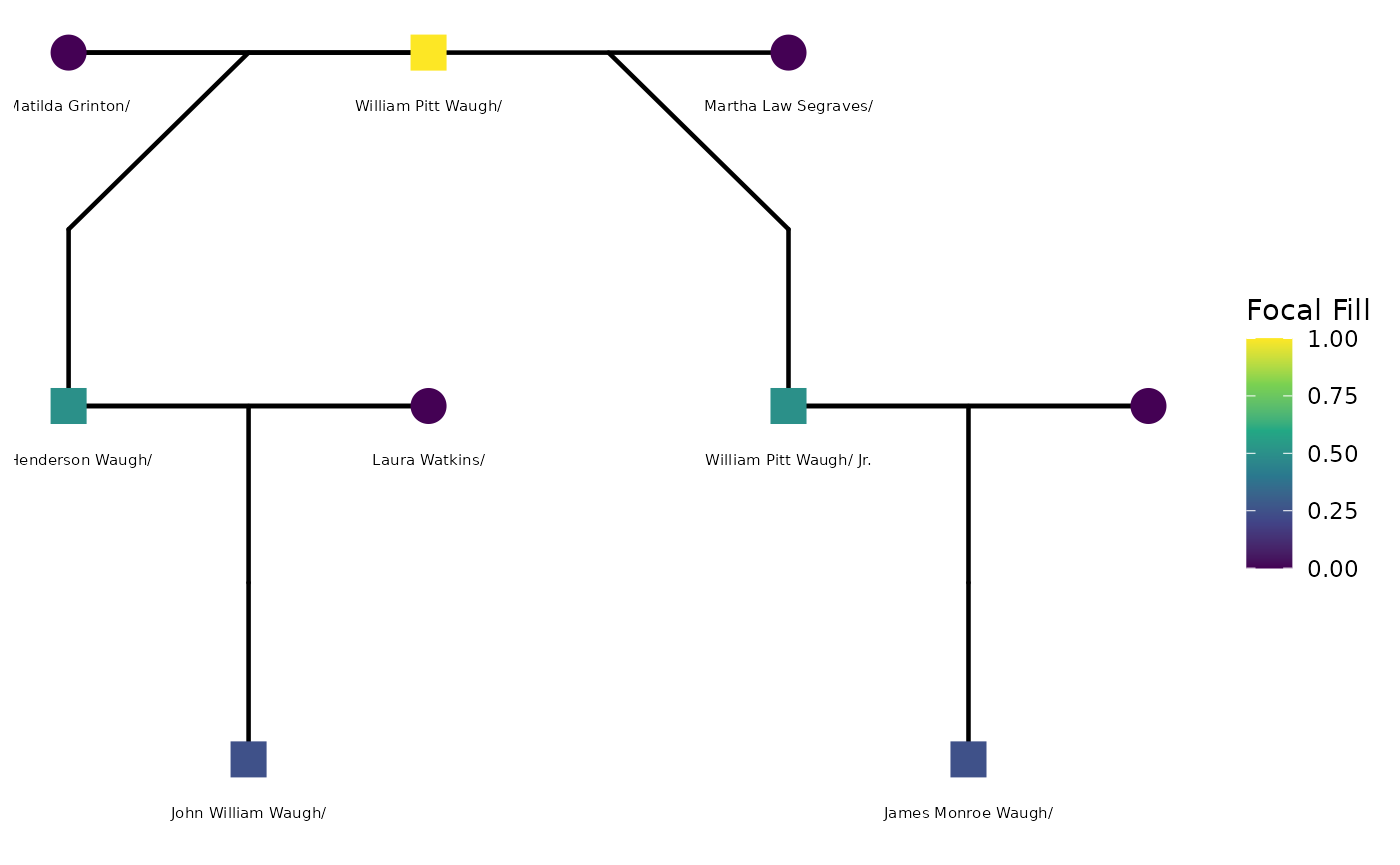
Please see the vignettes from the ggpedigree package for
more on customizing pedigree diagrams with
ggpedigree().
Cleaning up
unlink(tmp_ged)Summary of functions
| Function | Purpose |
|---|---|
readGedcom(file) |
Parse INDI blocks → one row per person |
readGedcomFamilies(file) |
Parse FAM blocks → one row per family |
summarizeGedcom(df) |
Coverage counts and percentages |
extractGedcomYear(x) |
Year from any GEDCOM date string |
convertGedcomCoords(df) |
Convert _lat/_long columns to decimal
degrees |
gedcomLon2Numeric(x) |
Convert a longitude string vector |