2 Introduction to ggplot2
In this chapter, we explore the power of ggplot2 within the tidyverse package suite for creating compelling visual representations of twin studies in behavior genetics. ggplot2’s layer-oriented approach to building data visualizations allows researchers to intuitively map out the complexities inherent in twin data, providing insights that are crucial for both hypothesis testing and exploratory data analysis.
2.1 Understanding ggplot2’s Grammar of Graphics
ggplot2 is a powerful data visualization package in R that is part of the tidyverse suite of packages. It is based on the grammar of graphics, a coherent system for describing and building visualizations. The grammar of graphics is based on the idea that a plot can be decomposed into a set of independent components, such as data, aesthetics, and geoms (geometric objects). By combining these components, ggplot2 allows for the creation of complex and informative visualizations that can be easily customized and extended.
The structure of the code for plots can be summarized as follows:
ggplot(data = [[dataset]],
     mapping = aes(x = [[x-variable]],
                   y = [[y-variable]])) +
   geom_xxx() +
   other options
Each component of the plot is added in layers. The ggplot() function initializes the plot, aes() specifies the aesthetic mappings (how variables are mapped to visual properties), and geom_xxx() adds a geometric object (points, lines, bars, etc.) to the plot. Additional layers can be added to further customize the plot, such as labels, titles, and themes. We’ll dive into these soon enough, but first, let’s walk through a simple example to illustrate the basic structure of a ggplot2 plot.
2.2 Case Study: Visualizing Twin Data
To make this more concrete, let’s consider an example using twin data on height from the OpenMX package, which is in the twinData data. These 3,808 pairs of twins are from the Australian National Health and Medical Research Council Twin Registry. The dataset contains information on the height, weight, and body mass index (BMI) of twins, along with their zygosity and other demographic information.
library(tidyverse)  # Load the tidyverse packages
library(OpenMx)    # Load the OpenMx package
library(BGmisc) # Load the BGmisc package
library(conflicted) # to handle conflicts
conflicted::conflicts_prefer(OpenMx::vech,dplyr::filter) # Resolve conflictsdata(twinData)
glimpse(twinData)
#> Rows: 3,808
#> Columns: 16
#> $ fam <int> 1, 2, 3, 4, 5, 6, 7, 8, 9, 10, 11, 12, 13, 14, 15, 16, 17, 18…
#> $ age <int> 21, 24, 21, 21, 19, 26, 23, 29, 24, 28, 29, 19, 23, 22, 23, 2…
#> $ zyg <int> 1, 1, 1, 1, 1, 1, 1, 1, 1, 1, 1, 1, 1, 1, 1, 1, 1, 1, 1, 1, 1…
#> $ part <int> 2, 2, 2, 2, 2, 2, 2, 2, 2, 2, 2, 2, 2, 2, 2, 2, 2, 2, 2, 2, 2…
#> $ wt1 <int> 58, 54, 55, 66, 50, 60, 65, 40, 60, 76, 48, 70, 51, 53, 58, 4…
#> $ wt2 <int> 57, 53, 50, 76, 48, 60, 65, 39, 57, 64, 51, 67, 51, 55, 57, 5…
#> $ ht1 <dbl> 1.70, 1.63, 1.65, 1.57, 1.61, 1.60, 1.75, 1.56, 1.76, 1.70, 1…
#> $ ht2 <dbl> 1.70, 1.63, 1.68, 1.65, 1.63, 1.57, 1.77, 1.53, 1.77, 1.73, 1…
#> $ htwt1 <dbl> 20.1, 20.3, 20.2, 26.8, 19.3, 23.4, 21.2, 16.4, 19.4, 26.3, 2…
#> $ htwt2 <dbl> 19.7, 19.9, 17.7, 27.9, 18.1, 24.3, 20.7, 16.7, 18.2, 21.4, 2…
#> $ bmi1 <dbl> 21.0, 21.1, 21.0, 23.0, 20.7, 22.1, 21.4, 19.6, 20.7, 22.9, 2…
#> $ bmi2 <dbl> 20.9, 21.0, 20.1, 23.3, 20.3, 22.3, 21.2, 19.7, 20.3, 21.4, 2…
#> $ cohort <chr> "younger", "younger", "younger", "younger", "younger", "young…
#> $ zygosity <fct> MZFF, MZFF, MZFF, MZFF, MZFF, MZFF, MZFF, MZFF, MZFF, MZFF, M…
#> $ age1 <int> 21, 24, 21, 21, 19, 26, 23, 29, 24, 28, 29, 19, 23, 22, 23, 2…
#> $ age2 <int> 21, 24, 21, 21, 19, 26, 23, 29, 24, 28, 29, 19, 23, 22, 23, 2…I’m going to tidy up the data a bit by renaming the columns and removing some unnecessary columns. I’ll also filter out any rows with missing values in the height columns. I’ve also added a column to represent the sex of the twins and their zygosity.
twinData_cleaned <- twinData %>%
  rename( # Rename columns
    family = fam,
    weight_t1 = wt1,
    weight_t2 = wt2,
    height_t1 = ht1,
    height_t2 = ht2,
    bmi_t1 = bmi1,
    bmi_t2 = bmi2,
    age_t1 = age1,
    age_t2 = age2,
    heightweight_t1 = htwt1,
    heightweight_t2 = htwt2) %>%
  select(-c(# Remove unnecessary columns
    part,
    zyg,
    age_t1,
    age_t2)) %>%
  filter(# Remove rows with missing values
    !is.na(height_t1),
    !is.na(height_t2)) %>%
  mutate( # Create new columns
    sex = case_when(zygosity %in% c("MZFF","DZFF") ~ "F",
                                zygosity %in% c("MZMM","DZMM") ~ "M",
                                TRUE ~ "OS"),
                    zyg = case_when(zygosity %in% c("MZFF","MZMM") ~ "MZ",
                                    zygosity %in% c("DZFF","DZMM","DZOS") ~ "DZ",
                                TRUE ~ NA_character_ ))

glimpse(twinData_cleaned)
#> Rows: 3,667
#> Columns: 14
#> $ family          <int> 1, 2, 3, 4, 5, 6, 7, 8, 9, 10, 11, 12, 13, 14, 15, 16,…
#> $ age             <int> 21, 24, 21, 21, 19, 26, 23, 29, 24, 28, 29, 19, 23, 22…
#> $ weight_t1       <int> 58, 54, 55, 66, 50, 60, 65, 40, 60, 76, 48, 70, 51, 53…
#> $ weight_t2       <int> 57, 53, 50, 76, 48, 60, 65, 39, 57, 64, 51, 67, 51, 55…
#> $ height_t1       <dbl> 1.70, 1.63, 1.65, 1.57, 1.61, 1.60, 1.75, 1.56, 1.76, …
#> $ height_t2       <dbl> 1.70, 1.63, 1.68, 1.65, 1.63, 1.57, 1.77, 1.53, 1.77, …
#> $ heightweight_t1 <dbl> 20.1, 20.3, 20.2, 26.8, 19.3, 23.4, 21.2, 16.4, 19.4, …
#> $ heightweight_t2 <dbl> 19.7, 19.9, 17.7, 27.9, 18.1, 24.3, 20.7, 16.7, 18.2, …
#> $ bmi_t1          <dbl> 21.0, 21.1, 21.0, 23.0, 20.7, 22.1, 21.4, 19.6, 20.7, …
#> $ bmi_t2          <dbl> 20.9, 21.0, 20.1, 23.3, 20.3, 22.3, 21.2, 19.7, 20.3, …
#> $ cohort          <chr> "younger", "younger", "younger", "younger", "younger",…
#> $ zygosity        <fct> MZFF, MZFF, MZFF, MZFF, MZFF, MZFF, MZFF, MZFF, MZFF, …
#> $ sex             <chr> "F", "F", "F", "F", "F", "F", "F", "F", "F", "F", "F",…
#> $ zyg             <chr> "MZ", "MZ", "MZ", "MZ", "MZ", "MZ", "MZ", "MZ", "MZ", …
The code structure for our plot would look like this:
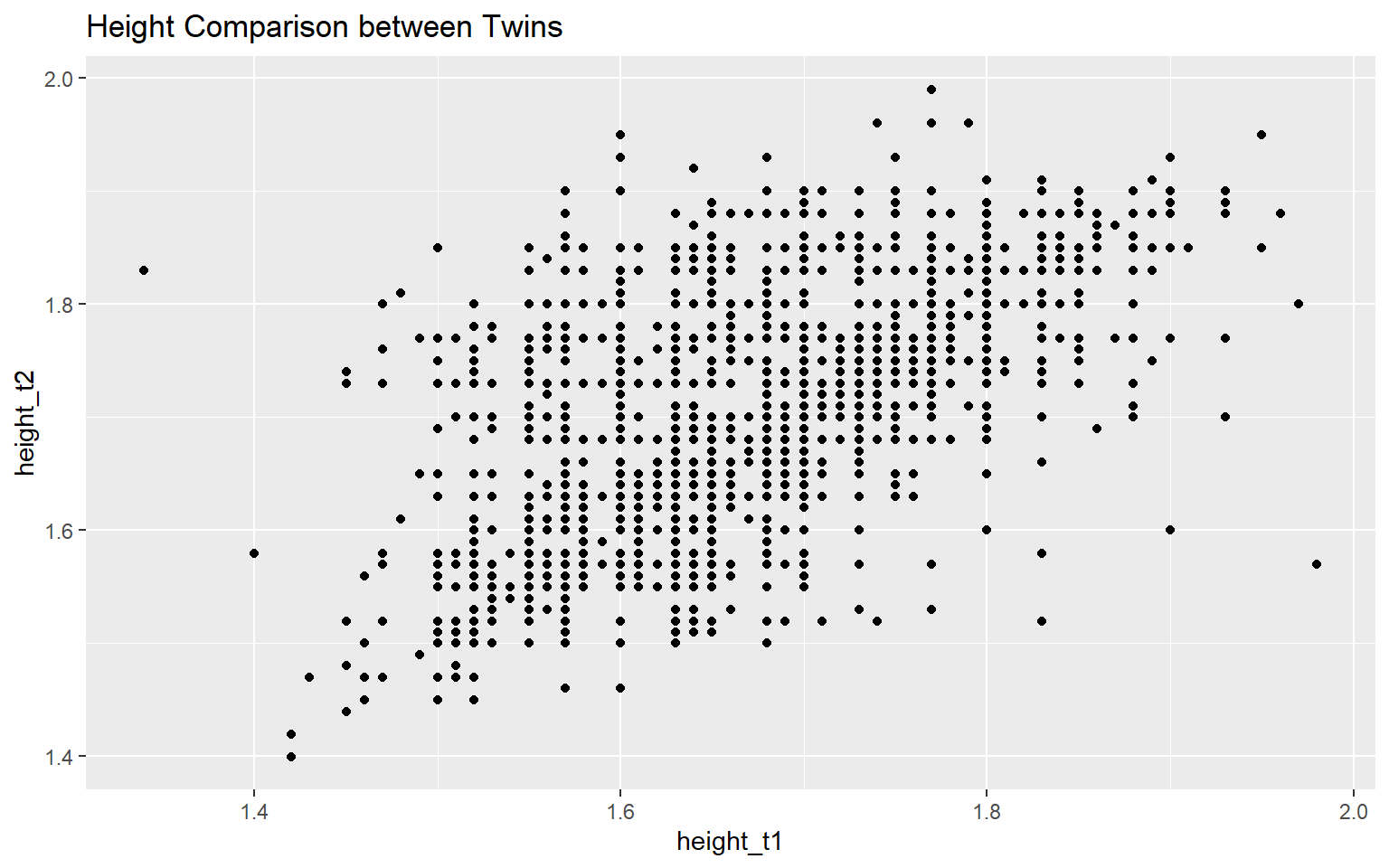
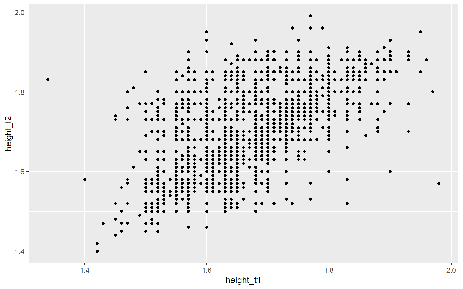
ggplot(data = twinData_cleaned, mapping = aes(x = height_t1,
                                              y = height_t2)) +
  geom_point() +
  labs(title = "Height Comparison between Twins")
It would produce a scatter plot comparing the height of twins with the height of twin 1 on the x-axis and the height of twin 2 on the y-axis.
2.2.1 Key Components of a ggplot2 Plot
The code above demonstrates the basic structure of a ggplot2 plot. To break down the key components of the plot you can press the left and right arrows on your keyboard to navigate through the slides below. Or if you prefer, you can click on the slide to advance to the next one. Below the slides you’ll find the same content in a more traditional format.
2.2.1.1 Plot Breakdown
Start with the twinData_cleaned data frame

Start with the twinData_cleaned data frame, map twin 1’s height to the x-axis
Start with the twinData_cleaned data frame, map twin 1’s height to the x-axis, and and map twin 2’s height to the y-axis.
Start with the twinData_cleaned data frame, map twin 1’s height to the x-axis, and and map twin 2’s height to the y-axis. Represent each observation with a point
Start with the twinData_cleaned data frame, map twin 1’s height to the x-axis, and and map twin 2’s height to the y-axis. Represent each observation with a point, and map zygosity to the color of each point.
ggplot(data = twinData_cleaned,
       mapping = aes( x = height_t1,
                      y = height_t2,
                      color = zyg)) + #<<
geom_point() 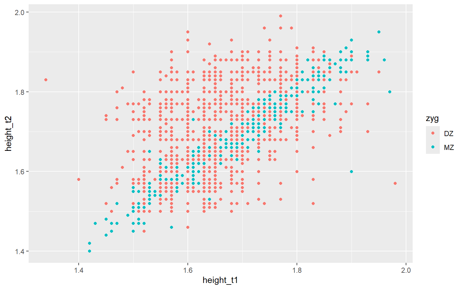
Start with the twinData_cleaned data frame, map twin 1’s height to the x-axis, and and map twin 2’s height to the y-axis. Represent each observation with a point, and map zygosity to the color of each point. Title the plot “Height Comparison between Twins”
ggplot(data = twinData_cleaned,
       mapping = aes( x = height_t1,
                      y = height_t2,
                      color = zyg)) +
  geom_point() +
  labs(title = "Height Comparison between Twins") #<<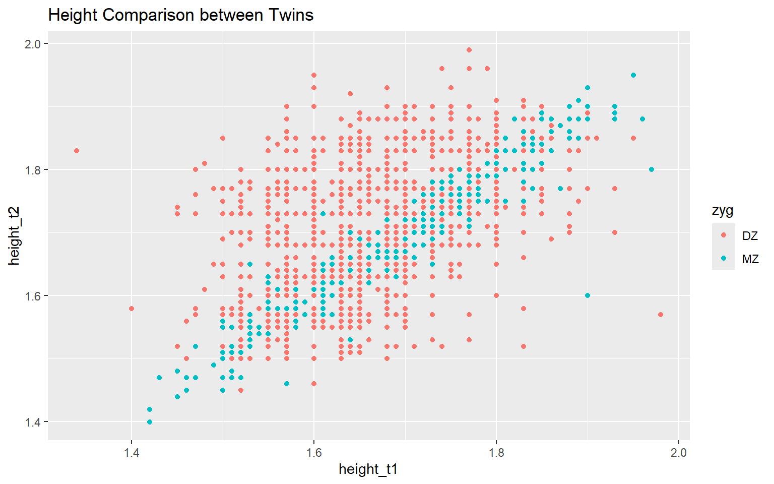
Start with the twinData_cleaned data frame, map twin 1’s height to the x-axis, and and map twin 2’s height to the y-axis. Represent each observation with a point, and map zygosity to the color of each point. Title the plot “Height Comparison between Twins”, add the subtitle “by zygosity”
ggplot(data = twinData_cleaned,
       mapping = aes( x = height_t1,
                      y = height_t2,
                      color = zyg)) +
  geom_point() +
  labs(title = "Height Comparison between Twins",
       subtitle = "by zygosity") #<<
Start with the twinData_cleaned data frame, map twin 1’s height to the x-axis, and and map twin 2’s height to the y-axis. Represent each observation with a point, and map zygosity to the color of each point. Title the plot “Height Comparison between Twins”, add the subtitle “by zygosity”, label the x and y axes as “Height of Twin 1 (m)” and “Height of Twin 2 (m)”, respectively
ggplot(data = twinData_cleaned,
       mapping = aes( x = height_t1,
                      y = height_t2,
                      color = zyg)) +
  geom_point() +
  labs(title = "Height Comparison between Twins",
       subtitle = "by zygosity",
       x = "Height of Twin 1 (m)", y = "Height of Twin 2 (m)") #<<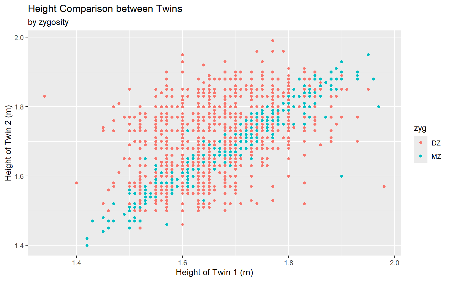
Start with the twinData_cleaned data frame, map twin 1’s height to the x-axis, and and map twin 2’s height to the y-axis. Represent each observation with a point, and map zygosity to the color of each point. Title the plot “Height Comparison between Twins”, add the subtitle “by zygosity”, label the x and y axes as “Height of Twin 1 (m)” and “Height of Twin 2 (m)”, respectively , label the legend “Zygosity”
ggplot(data = twinData_cleaned,
       mapping = aes( x = height_t1,
                      y = height_t2,
                      color = zyg)) +
  geom_point() +
  labs(title = "Height Comparison between Twins",
       subtitle = "by zygosity",
       x = "Height of Twin 1 (m)", y = "Height of Twin 2 (m)",
       color = "Zygosity") #<<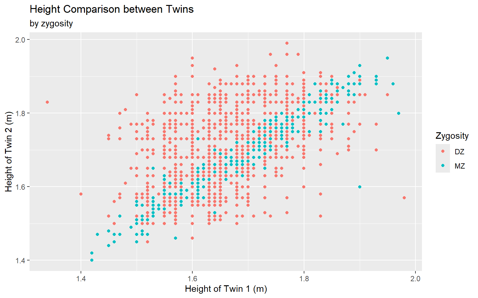
Start with the twinData_cleaned data frame, map twin 1’s height to the x-axis, and and map twin 2’s height to the y-axis. Represent each observation with a point, and map zygosity to the color of each point. Title the plot “Height Comparison between Twins”, add the subtitle “by zygosity”, label the x and y axes as “Height of Twin 1 (m)” and “Height of Twin 2 (m)”, respectively , label the legend “Zygosity”, and add a caption for the data source.
ggplot(data = twinData_cleaned,
       mapping = aes( x = height_t1,
                      y = height_t2,
                      color = zyg)) +
  geom_point() +
  labs(title = "Height Comparison between Twins",
       subtitle = "by zygosity",
       x = "Height of Twin 1 (m)", y = "Height of Twin 2 (m)",
       color = "Zygosity",
       caption = "Source: Australian National Health and Medical Research Council Twin Registry / OpenMx package") #<<
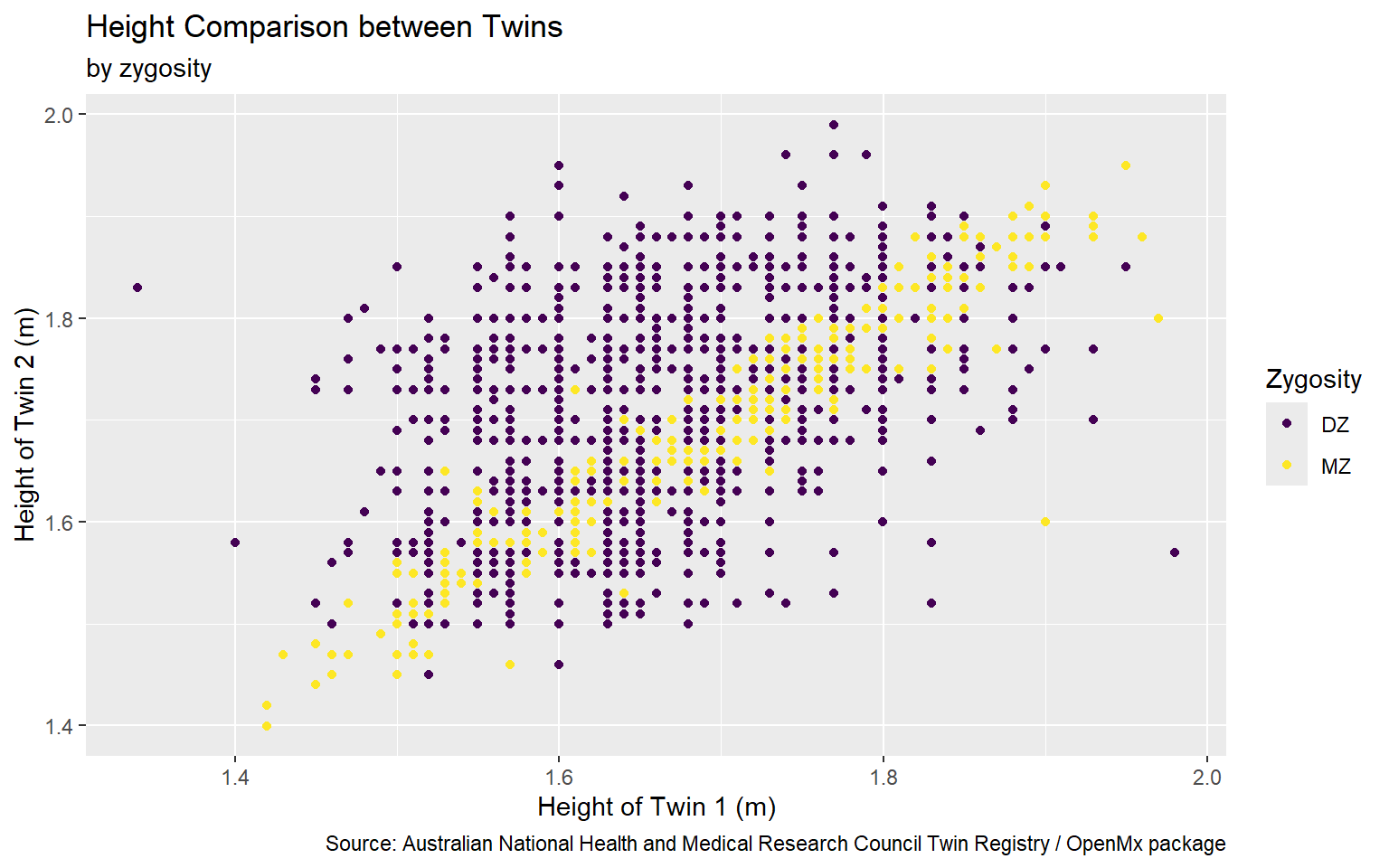
Start with the twinData_cleaned data frame, map twin 1’s height to the x-axis, and and map twin 2’s height to the y-axis. Represent each observation with a point, and map zygosity to the color of each point. Title the plot “Height Comparison between Twins”, add the subtitle “by zygosity”, label the x and y axes as “Height of Twin 1 (m)” and “Height of Twin 2 (m)”, respectively , label the legend “Zygosity”, and add a caption for the data source. Finally, use a discrete color scale that is designed to be perceived by viewers with common forms of color blindness.
ggplot(data = twinData_cleaned,
       mapping = aes( x = height_t1,
                      y = height_t2,
                      color = zyg)) +
  geom_point() +
  labs(title = "Height Comparison between Twins",
       subtitle = "by zygosity",
       x = "Height of Twin 1 (m)", y = "Height of Twin 2 (m)",
       color = "Zygosity",
       caption = "Source: Australian National Health and Medical Research Council Twin Registry / OpenMx package") +
  scale_color_viridis_d() #<<